एक्सेल में किसी मूल्य के सभी मिलान किए गए उदाहरणों को कैसे सूचीबद्ध करें?

लेखक: सिलुविया अंतिम संशोधित: 2020-06-04

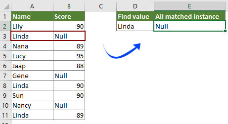
जैसा कि बाएं स्क्रीनशॉट में दिखाया गया है, आपको तालिका में मूल्य "लिंडा" के सभी मिलान उदाहरणों को ढूंढना और सूचीबद्ध करना होगा। उसकी प्राप्ति कैसे हो? कृपया इस आलेख में दिए गए तरीकों को आज़माएँ।

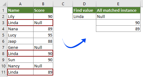
सरणी सूत्र के साथ किसी मान के सभी मिलान किए गए उदाहरणों को सूचीबद्ध करें
एक्सेल के लिए कुटूल के साथ किसी मान के केवल पहले मिलान वाले उदाहरण को आसानी से सूचीबद्ध करें
VLOOKUP के लिए अधिक ट्यूटोरियल...

सरणी सूत्र के साथ किसी मान के सभी मिलान किए गए उदाहरणों को सूचीबद्ध करें

निम्नलिखित सरणी सूत्र के साथ, आप एक्सेल में एक निश्चित तालिका में किसी मान के सभी मिलान उदाहरणों को आसानी से सूचीबद्ध कर सकते हैं। कृपया निम्नानुसार करें.

1. पहले मिलान किए गए उदाहरण को आउटपुट करने के लिए एक रिक्त सेल का चयन करें, इसमें नीचे दिया गया सूत्र दर्ज करें, और फिर दबाएं कंट्रोल + पाली + दर्ज एक साथ चाबियाँ।

=INDEX($B$2:$B$11, SMALL(IF($D$2=$A$2:$A$11, ROW($A$2:$A$11)-ROW($A$2)+1), ROW(1:1)))

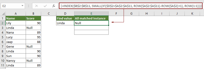
नोट: सूत्र में, B2:B11 वह श्रेणी है जिसमें मिलान किए गए उदाहरण स्थित होते हैं। A2:A11 वह श्रेणी है जिसमें वह निश्चित मान होता है जिसके आधार पर आप सभी उदाहरणों को सूचीबद्ध करेंगे। और D2 में निश्चित मान शामिल है।

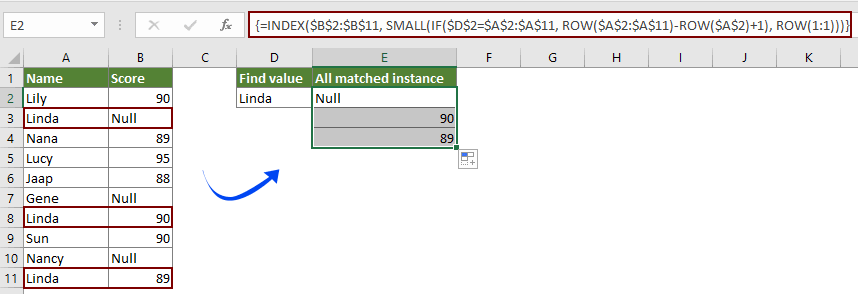
2. परिणाम सेल का चयन करते रहें, फिर अन्य मिलान किए गए उदाहरण प्राप्त करने के लिए भरण हैंडल को नीचे खींचें।

एक्सेल के लिए कुटूल के साथ किसी मान के केवल पहले मिलान वाले उदाहरण को आसानी से सूचीबद्ध करें

आप किसी मान के पहले मिलान वाले उदाहरण को आसानी से ढूंढ और सूचीबद्ध कर सकते हैं सूची में कोई मान खोजें के समारोह एक्सेल के लिए कुटूल बिना फॉर्मूलों को याद किये. कृपया निम्नानुसार करें.

आवेदन करने से पहले एक्सेल के लिए कुटूल, कृपया सबसे पहले इसे डाउनलोड करें और इंस्टॉल करें.

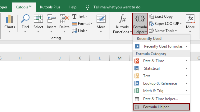
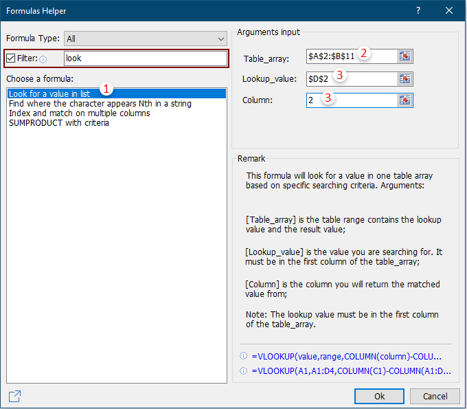
1. एक रिक्त कक्ष का चयन करें जिसमें आप पहले मिलान किए गए उदाहरण को रखेंगे, फिर क्लिक करें कुटूल > फॉर्मूला हेल्पर > फॉर्मूला हेल्पर.

2। में सूत्र सहायक संवाद बॉक्स, आपको यह करना होगा:

2.1 खोजें और चुनें सूची में कोई मान खोजें में विकल्प एक सूत्र चुनें डिब्बा;
टिप्स: आप जांच कर सकते हैं फ़िल्टर बॉक्स में, आपको आवश्यक फ़ॉर्मूले को तुरंत फ़िल्टर करने के लिए टेक्स्टबॉक्स में कीवर्ड दर्ज करें।

2.2 में तालिका सरणी बॉक्स, तालिका श्रेणी का चयन करें जिसमें विशिष्ट मान कॉलम और मिलान किए गए इंस्टेंस कॉलम दोनों शामिल हैं;

2.3 में लुक_वैल्यू बॉक्स में, उस विशिष्ट मान वाले सेल का चयन करें जिसके आधार पर आप पहला उदाहरण सूचीबद्ध करेंगे;

2.4 में स्तंभ बॉक्स में, मिलान किए गए उदाहरण वाले कॉलम का चयन करें। या बस इसमें कॉलम नंबर दर्ज करें;
टिप्स: कॉलम नंबर चयनित कॉलमों की संख्या पर आधारित है, यदि आप चार कॉलम चुनते हैं, और यह तीसरा कॉलम है, तो आपको नंबर 3 दर्ज करना होगा स्तंभ डिब्बा।

2.5 क्लिक करें OK बटन.

फिर दिए गए मान का पहला मिलान उदाहरण नीचे दिखाए गए स्क्रीनशॉट के अनुसार सूचीबद्ध किया गया है।

यदि आप इस उपयोगिता का निःशुल्क परीक्षण (30-दिन) चाहते हैं, कृपया इसे डाउनलोड करने के लिए क्लिक करें, और फिर उपरोक्त चरणों के अनुसार ऑपरेशन लागू करने के लिए जाएं।

सर्वोत्तम कार्यालय उत्पादकता उपकरण

🤖	कुटूल्स एआई सहयोगी: निम्न के आधार पर डेटा विश्लेषण में क्रांति लाएं: बुद्धिमान निष्पादन \| कोड जनरेट करें \| कस्टम फ़ॉर्मूले बनाएं \| डेटा का विश्लेषण करें और चार्ट बनाएं \| कुटूल फ़ंक्शंस का आह्वान करें...
	लोकप्रिय सुविधाएँ: डुप्लिकेट ढूंढें, हाइलाइट करें या पहचानें \| रिक्त पंक्तियाँ हटाएँ \| डेटा खोए बिना कॉलम या सेल को संयोजित करें \| फॉर्मूला के बिना गोल ...
	सुपर लुकअप: एकाधिक मानदंड VLookup \| मल्टीपल वैल्यू वीलुकअप \| अनेक शीटों में VLookup \| फजी लुकअप ....
	उन्नत ड्रॉप-डाउन सूची: शीघ्रता से ड्रॉप डाउन सूची बनाएं \| आश्रित ड्रॉप डाउन सूची \| बहु-चयन ड्रॉप डाउन सूची ....
	स्तम्भ प्रबंधक: कॉलमों की एक विशिष्ट संख्या जोड़ें \| कॉलम ले जाएँ \| छिपे हुए कॉलम की दृश्यता स्थिति टॉगल करें \| रेंज और कॉलम की तुलना करें ...
	फीचर्ड फीचर्स: ग्रिड फोकस \| डिजाइन देखें \| बड़ा फॉर्मूला बार \| कार्यपुस्तिका एवं शीट प्रबंधक \| संसाधन लाइब्रेरी (ऑटो टेक्स्ट) \| खजूर बीनने वाला \| कार्यपत्रकों को संयोजित करें \| एन्क्रिप्ट/डिक्रिप्ट सेल \| सूची के अनुसार ईमेल भेजें \| सुपर फ़िल्टर \| विशेष फ़िल्टर (फ़िल्टर बोल्ड/इटैलिक/स्ट्राइकथ्रू...) ...
	शीर्ष 15 टूलसेट: 12 टेक्स्ट टूल्स (पाठ जोड़ें, अक्षर हटाएँ, ...) \| 50 + चार्ट प्रकार (गैन्ट चार्ट, ...) \| 40+ प्रैक्टिकल सूत्र (जन्मदिन के आधार पर आयु की गणना करें, ...) \| 19 निवेशन टूल्स (QR कोड डालें, पथ से चित्र सम्मिलित करें, ...) \| 12 रूपांतरण टूल्स (शब्दों को संख्याएँ, मुद्रा रूपांतरण, ...) \| 7 विलय और विभाजन टूल्स (उन्नत संयोजन पंक्तियाँ, विभाजन कोशिकाओं, ...) \| ... और अधिक

एक्सेल के लिए कुटूल के साथ अपने एक्सेल कौशल को सुपरचार्ज करें, और पहले जैसी दक्षता का अनुभव करें। एक्सेल के लिए कुटूल उत्पादकता बढ़ाने और समय बचाने के लिए 300 से अधिक उन्नत सुविधाएँ प्रदान करता है। वह सुविधा प्राप्त करने के लिए यहां क्लिक करें जिसकी आपको सबसे अधिक आवश्यकता है...

Description

अधिक पढ़ें... मुफ्त डाउनलोड...

ऑफिस टैब ऑफिस में टैब्ड इंटरफ़ेस लाता है, और आपके काम को बहुत आसान बनाता है

Word, Excel, PowerPoint में टैब्ड संपादन और रीडिंग सक्षम करें, प्रकाशक, एक्सेस, विसियो और प्रोजेक्ट।
नई विंडो के बजाय एक ही विंडो के नए टैब में एकाधिक दस्तावेज़ खोलें और बनाएं।
आपकी उत्पादकता 50% बढ़ जाती है, और आपके लिए हर दिन सैकड़ों माउस क्लिक कम हो जाते हैं!

अधिक पढ़ें... मुफ्त डाउनलोड...

Comments (15)

Rated 5 out of 5 · 1 ratings

Brandon Beastall04

about 1 year ago

#43151

This comment was minimized by the moderator on the site

Is there a way to make it totla up the values it find and just put it in the first box?

Report

crystal Brandon Beastall04

about 1 year ago

#43183

This comment was minimized by the moderator on the site

Hi Bramdon,

To total up all matched values, the following formula can help. Or you can take a look at this tutorial: vlookup and sum matches in rows or columns in Excel
=SUMPRODUCT((A2:A7=A10)*B2:F7)

https://www.extendoffice.com/images/stories/doc-excel/doc-vlookup-and-sum/doc-vlookup-sum-sumif4.png

Report

Steven Waddleton

about 1 year ago

#40832

This comment was minimized by the moderator on the site

Is there a way to stop this formula returning duplicate values

Thanks
Steven

crystal Steven Waddleton

about 1 year ago

#40867

This comment was minimized by the moderator on the site

Hi Steven Waddleton,
The following two formulas can do you a favor.
Array formula in E2:
=INDEX($B$2:$B$11,MATCH(0,COUNTIF($E$1:E1,$B$2:$B$11)+($A$2:$A$11<>$D$2),0)) + Ctrl + Shift + Enter
Formula in E2:
=LOOKUP(2, 1/((COUNTIF($F$1:F1,$B$2:$B$11)=0)*($D$2=$A$2:$A$11)), $B$2:$B$11)
In the formulas, E1 is the cell above the result cell.

https://www.extendoffice.com/images/stories/comments/comment-picture-zxm/instance-no-duplicates.png

Report

Paolo Cavalli

about 1 year ago

#39528

This comment was minimized by the moderator on the site

WOW! Worked perfectly, thanks a ton! Awesome formula.

Rated 5 out of 5

Ton

about 2 years ago

#36380

This comment was minimized by the moderator on the site

Nice formula. In testing it I get #NUMBER! when I clear cells A9:B11. How to change the formula to prevent getting this error? I wonder, because I want to use this formula for a list of events on a certain date and on date 1 there are 40 events, on day 2 it are 10 events etc. I could create an indexed list for perhaps 100 rows, but it looks very strange when for date 2 the first 10 rows show events and the other 90 rows show #NUMBER!. It would be okay for me if it gave "-" as a result instead of #NUMBER!

Dev

about 2 years ago

#36216

This comment was minimized by the moderator on the site

Fantastic. Thank you so much. Very helpful for my work.

Gandhi, Shreepad

about 2 years ago

#35753

This comment was minimized by the moderator on the site

Amazing. The formula worked for me exactly the way I was looking for. Hats off. Thanks a ton

ChiTriGuy

about 3 years ago

#34219

This comment was minimized by the moderator on the site

Question, I have a sheet laid out opposite of this where "Linda" would be the column header I would like to flag on and the value "90" or 89" I would like to return. Would I change the row function to a column function?

Report

Luke

about 3 years ago

#34041

This comment was minimized by the moderator on the site

How would I use this formula but instead of filling down I could fill across but the formula would continue moving down as I fill across (ie. the formula changes from ROW(1:1) to ROW(2:2)

crystal Luke

about 3 years ago

#34042

This comment was minimized by the moderator on the site

Hi Luke,The below array formula can do you a favor. Note: After entering the formula, please press the Ctrl + Shift + Enter key to apply it. And then drag its Fill Handle right across the cells you need. =INDEX($B$2:$B$11, SMALL(IF($D$2=$A$2:$A$11, ROW($A$2:$A$11)-ROW($A$2)+1), COLUMN(A1)))

Report

Reggie100

about 4 years ago

#29931

This comment was minimized by the moderator on the site

A very useful and educational formula. I am matching against a set numeric value and it works a treat. How can I use >= rather than just = (i.e. IF($D$2>=$A$2:$A$11) to perform the match so it is looking for values greater than a set value (in $D$2). I assume as it doesn't work as one of the functions in the formula is matching against specific text rather than working with numbers?

Report

jmedina202

about 5 years ago

#28667

This comment was minimized by the moderator on the site

This was super useful, thanks! I'm trying to take this one step further and be able to return all match instances of a certain value while having to search through more than a single-column array. To work through this using your example, I added a second column of test scores and modified your formula to look up a given test score and return the names that match that score. I got this to work with INDEX(SMALL()) and can pull all of the names from both test columns. I've also managed to return only names with that score on Test 2 using INDEX(MATCH(INDEX(MATCH))), however this can only find the first instance in the array. What I'm really trying to do is a combination of these: return all of the names with the given array, while narrowing the search to a specific column within the array. Do you have any tips for this?

Report

crystal jmedina202

about 5 years ago

#28668

This comment was minimized by the moderator on the site

Good day,
Would you please provide a screenshot of your spreadsheet showing what you are exactly trying to do? Thank you for your comment.

Report

There are no comments posted here yet

Please leave your comments in English

Posting as Guest

Name (Required)

Email (Required)

Rate this post:

Reset

0 Characters

🤖	कुटूल्स एआई सहयोगी: निम्न के आधार पर डेटा विश्लेषण में क्रांति लाएं: बुद्धिमान निष्पादन \| कोड जनरेट करें \| कस्टम फ़ॉर्मूले बनाएं \| डेटा का विश्लेषण करें और चार्ट बनाएं \| कुटूल फ़ंक्शंस का आह्वान करें...
	लोकप्रिय सुविधाएँ: डुप्लिकेट ढूंढें, हाइलाइट करें या पहचानें \| रिक्त पंक्तियाँ हटाएँ \| डेटा खोए बिना कॉलम या सेल को संयोजित करें \| फॉर्मूला के बिना गोल ...
	सुपर लुकअप: एकाधिक मानदंड VLookup \| मल्टीपल वैल्यू वीलुकअप \| अनेक शीटों में VLookup \| फजी लुकअप ....
	उन्नत ड्रॉप-डाउन सूची: शीघ्रता से ड्रॉप डाउन सूची बनाएं \| आश्रित ड्रॉप डाउन सूची \| बहु-चयन ड्रॉप डाउन सूची ....
	स्तम्भ प्रबंधक: कॉलमों की एक विशिष्ट संख्या जोड़ें \| कॉलम ले जाएँ \| छिपे हुए कॉलम की दृश्यता स्थिति टॉगल करें \| रेंज और कॉलम की तुलना करें ...
	फीचर्ड फीचर्स: ग्रिड फोकस \| डिजाइन देखें \| बड़ा फॉर्मूला बार \| कार्यपुस्तिका एवं शीट प्रबंधक \| संसाधन लाइब्रेरी (ऑटो टेक्स्ट) \| खजूर बीनने वाला \| कार्यपत्रकों को संयोजित करें \| एन्क्रिप्ट/डिक्रिप्ट सेल \| सूची के अनुसार ईमेल भेजें \| सुपर फ़िल्टर \| विशेष फ़िल्टर (फ़िल्टर बोल्ड/इटैलिक/स्ट्राइकथ्रू...) ...
	शीर्ष 15 टूलसेट: 12 टेक्स्ट टूल्स (पाठ जोड़ें, अक्षर हटाएँ, ...) \| 50 + चार्ट प्रकार (गैन्ट चार्ट, ...) \| 40+ प्रैक्टिकल सूत्र (जन्मदिन के आधार पर आयु की गणना करें, ...) \| 19 निवेशन टूल्स (QR कोड डालें, पथ से चित्र सम्मिलित करें, ...) \| 12 रूपांतरण टूल्स (शब्दों को संख्याएँ, मुद्रा रूपांतरण, ...) \| 7 विलय और विभाजन टूल्स (उन्नत संयोजन पंक्तियाँ, विभाजन कोशिकाओं, ...) \| ... और अधिक