मुख्य सामग्री पर जाएं

एक्सेल टेबल से एकाधिक कॉलम वापस करने के लिए वीलुकअप कैसे करें?

लेखक: ज़ियाओयांग अंतिम संशोधित: 2020-12-25

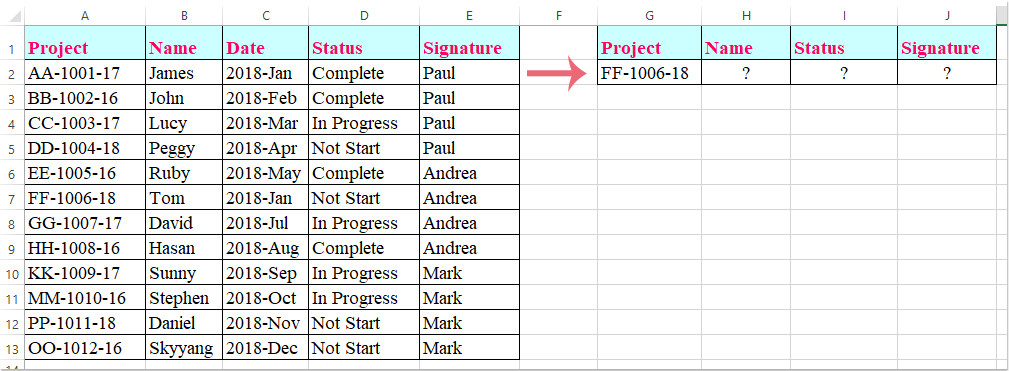
एक्सेल वर्कशीट में, आप एक कॉलम से मिलान मूल्य वापस करने के लिए Vlookup फ़ंक्शन लागू कर सकते हैं। लेकिन, कभी-कभी, आपको निम्नलिखित स्क्रीनशॉट में दिखाए गए अनुसार एकाधिक कॉलम से मिलान किए गए मान निकालने की आवश्यकता हो सकती है। Vlookup फ़ंक्शन का उपयोग करके आप एक ही समय में एकाधिक कॉलम से संबंधित मान कैसे प्राप्त कर सकते हैं?

दस्तावेज़ vlookup एकाधिक कॉलम 1

सरणी सूत्र के साथ एकाधिक स्तंभों से मिलान मान लौटाने के लिए Vlookup


सरणी सूत्र के साथ एकाधिक स्तंभों से मिलान मान लौटाने के लिए Vlookup

यहां, मैं एकाधिक कॉलम से मिलान किए गए मान वापस करने के लिए Vlookup फ़ंक्शन पेश करूंगा, कृपया इसे इस प्रकार करें:

1. उन कक्षों का चयन करें जहां आप एकाधिक स्तंभों से मेल खाने वाले मान रखना चाहते हैं, स्क्रीनशॉट देखें:

दस्तावेज़ vlookup एकाधिक कॉलम 2

2. फिर यह सूत्र दर्ज करें: =VLOOKUP(G2,A1:E13,{2,4,5},FALSE) सूत्र पट्टी में, और फिर दबाएँ Ctrl + Shift + Enter कुंजियाँ एक साथ, और कई कॉलमों से मेल खाने वाले मान एक साथ निकाले गए हैं, स्क्रीनशॉट देखें:

दस्तावेज़ vlookup एकाधिक कॉलम 3

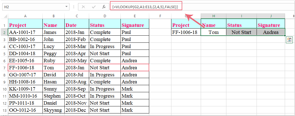
नोट: उपरोक्त सूत्र में, G2 वह मानदंड है जिसके आधार पर आप मान लौटाना चाहते हैं, ए1:ई13 वह तालिका श्रेणी है जिसे आप देखना चाहते हैं, संख्या 2, 4, 5 वे कॉलम संख्याएँ हैं जिनसे आप मान वापस करना चाहते हैं।

सर्वोत्तम कार्यालय उत्पादकता उपकरण

🤖 कुटूल्स एआई सहयोगी: निम्न के आधार पर डेटा विश्लेषण में क्रांति लाएं: बुद्धिमान निष्पादन   |  कोड जनरेट करें  |  कस्टम फ़ॉर्मूले बनाएं  |  डेटा का विश्लेषण करें और चार्ट बनाएं  |  कुटूल फ़ंक्शंस का आह्वान करें...
लोकप्रिय सुविधाएँ: डुप्लिकेट ढूंढें, हाइलाइट करें या पहचानें   |  रिक्त पंक्तियाँ हटाएँ   |  डेटा खोए बिना कॉलम या सेल को संयोजित करें   |   फॉर्मूला के बिना गोल ...
सुपर लुकअप: एकाधिक मानदंड VLookup    मल्टीपल वैल्यू वीलुकअप  |   अनेक शीटों में VLookup   |   फजी लुकअप ....
उन्नत ड्रॉप-डाउन सूची: शीघ्रता से ड्रॉप डाउन सूची बनाएं   |  आश्रित ड्रॉप डाउन सूची   |  बहु-चयन ड्रॉप डाउन सूची ....
स्तम्भ प्रबंधक: कॉलमों की एक विशिष्ट संख्या जोड़ें  |  कॉलम ले जाएँ  |  छिपे हुए कॉलम की दृश्यता स्थिति टॉगल करें  |  रेंज और कॉलम की तुलना करें ...
फीचर्ड फीचर्स: ग्रिड फोकस   |  डिजाइन देखें   |   बड़ा फॉर्मूला बार    कार्यपुस्तिका एवं शीट प्रबंधक   |  संसाधन लाइब्रेरी (ऑटो टेक्स्ट)   |  खजूर बीनने वाला   |  कार्यपत्रकों को संयोजित करें   |  एन्क्रिप्ट/डिक्रिप्ट सेल    सूची के अनुसार ईमेल भेजें   |  सुपर फ़िल्टर   |   विशेष फ़िल्टर (फ़िल्टर बोल्ड/इटैलिक/स्ट्राइकथ्रू...) ...
शीर्ष 15 टूलसेट12 टेक्स्ट टूल्स (पाठ जोड़ें, अक्षर हटाएँ, ...)   |   50 + चार्ट प्रकार (गैन्ट चार्ट, ...)   |   40+ प्रैक्टिकल सूत्र (जन्मदिन के आधार पर आयु की गणना करें, ...)   |   19 निवेशन टूल्स (QR कोड डालें, पथ से चित्र सम्मिलित करें, ...)   |   12 रूपांतरण टूल्स (शब्दों को संख्याएँ, मुद्रा रूपांतरण, ...)   |   7 विलय और विभाजन टूल्स (उन्नत संयोजन पंक्तियाँ, विभाजन कोशिकाओं, ...)   |   ... और अधिक

एक्सेल के लिए कुटूल के साथ अपने एक्सेल कौशल को सुपरचार्ज करें, और पहले जैसी दक्षता का अनुभव करें। एक्सेल के लिए कुटूल उत्पादकता बढ़ाने और समय बचाने के लिए 300 से अधिक उन्नत सुविधाएँ प्रदान करता है।  वह सुविधा प्राप्त करने के लिए यहां क्लिक करें जिसकी आपको सबसे अधिक आवश्यकता है...

Description


ऑफिस टैब ऑफिस में टैब्ड इंटरफ़ेस लाता है, और आपके काम को बहुत आसान बनाता है

  • Word, Excel, PowerPoint में टैब्ड संपादन और रीडिंग सक्षम करें, प्रकाशक, एक्सेस, विसियो और प्रोजेक्ट।
  • नई विंडो के बजाय एक ही विंडो के नए टैब में एकाधिक दस्तावेज़ खोलें और बनाएं।
  • आपकी उत्पादकता 50% बढ़ जाती है, और आपके लिए हर दिन सैकड़ों माउस क्लिक कम हो जाते हैं!
Comments (15)
No ratings yet. Be the first to rate!
This comment was minimized by the moderator on the site
how can i search for multiple lookup value?for eg: these two arrays shows diff freq coumn,gain,veritcal BW,tolerance etc.I want to get an average values gain and 3db BW..how can i enter the formula
y1    1800    7.5dBi +/- 2.9    22.1° +/- 6.8        7.5
y1    1900    7.6dBi +/- 3.0    18.9° +/- 3.6        7.6
y1    2100    6.7dBi +/- 2.6    17.7° +/- 3.6        6.7
y1    AWS    7.2dBi +/- 2.8    20.4° +/- 9.4        7.2
y1    2300    8.3dBi +/- 3.6    15.8° +/- 1.6        8.3
y1    2600    7.9dBi +/- 2.4    17.1° +/- 1.7        7.9
y2    1800    6.9dBi +/- 1.4    27.1° +/- 10.8        6.9
y2    1900    6.9dBi +/- 1.5    23.0° +/- 12.5        6.9
y2    2100    7.6dBi +/- 2.3    21.7° +/- 19.6        7.6
y2    AWS    8.0dBi +/- 2.5    23.3° +/- 13.8        8
y2    2300    7.7dBi +/- 1.6    15.9° +/- 5.9        7.7
y2    2600    6.5dBi +/- 2.3    14.5° +/- 3.9        6.5
This comment was minimized by the moderator on the site
I have many rows with same value but need to get multiple value after look up, I need to get two different EO ref , how can U##TRX EO
HXPRE-MQ1371 AB0024822
This comment was minimized by the moderator on the site
Thank you!! The { } of the columns is what I was missing. Appreciate this page!
This comment was minimized by the moderator on the site
Thanks! Super helpful, when other online options weren't
This comment was minimized by the moderator on the site
What if you need to have multiple rows as well? Ex. find all the FF-1006-18 rows while still only bringing back column B, D, and E.
This comment was minimized by the moderator on the site
Hello, Shelly,
Maybe there is not a direct formula for helping you, but, you can apply the below array fromula to get all matching values from the entire row, and then delete or hide the unwanted column as you need.
=INDEX($A$2:$E$10, SMALL(IF($G$2=$A$2:$A$10, ROW($A$2:$A$10)-MIN(ROW($A$2:$A$10))+1, ""), ROW(B1)),COLUMN(B1))
Then press Ctrl + Shift + Enter keys to get the first cell and then drag the fill handle to right and then drga down to get all corresponding values.

Please try, hope it can help you!
This comment was minimized by the moderator on the site
Thanks! This was really Helpful!
This comment was minimized by the moderator on the site
This method does not work. Even if it did, it is not the proper method.
Example of correct method is:
VLOOKUP($A2:$A1093, '[Workbook1.xlsx]Sheet2'!$A$2:$D$111,COLUMN(G2),FALSE)

Make sure you add $ before the column letter of your lookup reference to make sure it remains static, once done, using the filler button on the selected target cell, drag right to the corresponding number of columns.
This comment was minimized by the moderator on the site
This comment is exactly what I needed
This comment was minimized by the moderator on the site
How can I do this using 2 different spread sheets?
This comment was minimized by the moderator on the site
Hello, Lana,
The above formula in this article also can help you to get the results in another worksheet, you just need to change the cell reference as follows:
=VLOOKUP(A1,Sheet1!A1:E13,{2,4,5},FALSE)
Please remember to press Ctrl + Shift + Enter keys together to get the correct results.
This comment was minimized by the moderator on the site
NOT GETTING MULTIPLE COLUMN I'M GETTING ONLY ONE COLUMN VALUE
This comment was minimized by the moderator on the site
Hi, HARI,
To apply this formula, first, you should select the multiple cells where you want to output the results, and then copy the formula into the formula bar, then press Ctrl + Shift + Enter keys together to get the results.
Please try, hope it can help you!
This comment was minimized by the moderator on the site
This is great. How do I carry this formula down if I have 10,000 rows? I've tried a few ways but of course it's changing the formula on me.
This comment was minimized by the moderator on the site
Hi, Scully,
To apply this formula to multiple rows, you just need to change the relative cell reference to absolute reference, as this: =VLOOKUP(A1,Sheet1!$A$1:$E$13,{2,4,5},FALSE).
Please try this, hope it can help you!
There are no comments posted here yet
Please leave your comments in English
Posting as Guest
×
Rate this post:
0   Characters
Suggested Locations