एक्सेल में एक सेल में एकाधिक मान वापस करने के लिए वीलुकअप कैसे करें?
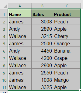
आम तौर पर, एक्सेल में, जब आप VLOOKUP फ़ंक्शन का उपयोग करते हैं, यदि मानदंड से मेल खाने के लिए कई मान हैं, तो आप केवल पहला मान प्राप्त कर सकते हैं। लेकिन, कभी-कभी, आप मानदंडों को पूरा करने वाले सभी संबंधित मानों को एक सेल में वापस करना चाहते हैं जैसा कि स्क्रीनशॉट में दिखाया गया है, आप इसे कैसे हल कर सकते हैं?
TEXTJOIN फ़ंक्शन (Excel 2019 और Office 365) के साथ एक सेल में एकाधिक मान लौटाने के लिए Vlookup
- सभी मेल खाने वाले मानों को एक सेल में वापस करने के लिए Vlookup
- Vlookup सभी मिलान मानों को डुप्लिकेट के बिना एक सेल में वापस करने के लिए
उपयोगकर्ता परिभाषित फ़ंक्शन के साथ एक सेल में एकाधिक मान लौटाने के लिए Vlookup
- सभी मेल खाने वाले मानों को एक सेल में वापस करने के लिए Vlookup
- Vlookup सभी मिलान मानों को डुप्लिकेट के बिना एक सेल में वापस करने के लिए
एक उपयोगी सुविधा के साथ एक सेल में एकाधिक मान लौटाने के लिए Vlookup
TEXTJOIN फ़ंक्शन (Excel 2019 और Office 365) के साथ एक सेल में एकाधिक मान लौटाने के लिए Vlookup
यदि आपके पास Excel का उच्च संस्करण जैसे Excel 2019 और Office 365 है, तो एक नया फ़ंक्शन है - टेक्स्टजॉइन, इस शक्तिशाली फ़ंक्शन के साथ, आप जल्दी से वीलुकअप कर सकते हैं और सभी मिलान मानों को एक सेल में वापस कर सकते हैं।
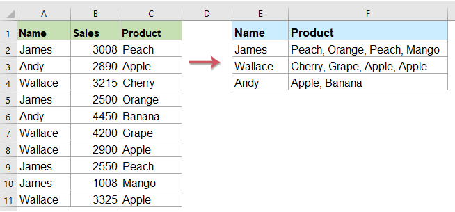
सभी मेल खाने वाले मानों को एक सेल में वापस करने के लिए Vlookup
कृपया नीचे दिए गए सूत्र को रिक्त कक्ष में लागू करें जहां आप परिणाम डालना चाहते हैं, फिर दबाएँ Ctrl + Shift + Enter पहला परिणाम प्राप्त करने के लिए कुंजियाँ एक साथ रखें, और फिर भरण हैंडल को उस सेल तक खींचें, जहाँ आप इस सूत्र का उपयोग करना चाहते हैं, और आपको नीचे दिखाए गए स्क्रीनशॉट के अनुसार सभी संबंधित मान प्राप्त होंगे:
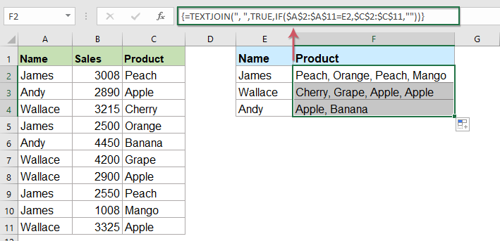
Vlookup सभी मिलान मानों को डुप्लिकेट के बिना एक सेल में वापस करने के लिए
यदि आप डुप्लिकेट के बिना लुकअप डेटा के आधार पर सभी मिलान मान वापस करना चाहते हैं, तो नीचे दिया गया सूत्र आपकी मदद कर सकता है।
कृपया निम्नलिखित सूत्र को कॉपी करके एक रिक्त कक्ष में चिपकाएँ, फिर दबाएँ Ctrl + Shift + Enter पहला परिणाम प्राप्त करने के लिए कुंजियाँ एक साथ रखें, और फिर अन्य कक्षों को भरने के लिए इस सूत्र को कॉपी करें, और आपको डुप्लिकेट वाले बिना सभी संबंधित मान प्राप्त होंगे जैसा कि नीचे स्क्रीनशॉट में दिखाया गया है:
उपयोगकर्ता परिभाषित फ़ंक्शन के साथ एक सेल में एकाधिक मान लौटाने के लिए Vlookup
उपरोक्त TEXTJOIN फ़ंक्शन केवल Excel 2019 और Office 365 के लिए उपलब्ध है, यदि आपके पास अन्य निम्न Excel संस्करण हैं, तो आपको इस कार्य को पूरा करने के लिए कुछ कोड का उपयोग करना चाहिए।
सभी मेल खाने वाले मानों को एक सेल में वापस करने के लिए Vlookup
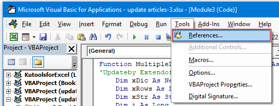
1. दबाए रखें ALT + F11 कुंजियाँ, और यह खुल जाती है अनुप्रयोगों के लिए माइक्रोसॉफ्ट विज़ुअल बेसिक खिड़की.
2। क्लिक करें सम्मिलित करें > मॉड्यूल, और निम्नलिखित कोड को इसमें पेस्ट करें मॉड्यूल विंडो.
वीबीए कोड: एक सेल में एकाधिक मान लौटाने के लिए Vlookup
Function ConcatenateIf(CriteriaRange As Range, Condition As Variant, ConcatenateRange As Range, Optional Separator As String = ",") As Variant
'Updateby Extendoffice
Dim xResult As String
On Error Resume Next
If CriteriaRange.Count <> ConcatenateRange.Count Then
    ConcatenateIf = CVErr(xlErrRef)
    Exit Function
End If
For i = 1 To CriteriaRange.Count
    If CriteriaRange.Cells(i).Value = Condition Then
        xResult = xResult & Separator & ConcatenateRange.Cells(i).Value
    End If
Next i
If xResult <> "" Then
    xResult = VBA.Mid(xResult, VBA.Len(Separator) + 1)
End If
ConcatenateIf = xResult
Exit Function
End Function
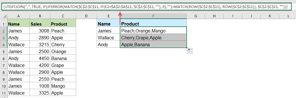
3. फिर इस कोड को सहेजें और बंद करें, वर्कशीट पर वापस जाएं और यह सूत्र दर्ज करें: =CONCATENATEIF($A$2:$A$11, E2, $C$2:$C$11, ", ") एक विशिष्ट रिक्त सेल में जहां आप परिणाम रखना चाहते हैं, फिर एक सेल में सभी संबंधित मान प्राप्त करने के लिए भरण हैंडल को नीचे खींचें, स्क्रीनशॉट देखें:
Vlookup सभी मिलान मानों को डुप्लिकेट के बिना एक सेल में वापस करने के लिए
लौटाए गए मिलान मानों में डुप्लिकेट को अनदेखा करने के लिए, कृपया नीचे दिए गए कोड का उपयोग करें।
1. दबाए रखें ऑल्ट + F11 कुंजी को खोलने के लिए अनुप्रयोगों के लिए माइक्रोसॉफ्ट विज़ुअल बेसिक खिड़की.
2। क्लिक करें सम्मिलित करें > मॉड्यूल, और निम्नलिखित कोड को इसमें पेस्ट करें मॉड्यूल विंडो.
वीबीए कोड: वीलुकअप और एक सेल में कई अद्वितीय मिलान वाले मान लौटाएं
Function MultipleLookupNoRept(Lookupvalue As String, LookupRange As Range, ColumnNumber As Integer)
'Updateby Extendoffice
    Dim xDic As New Dictionary
    Dim xRows As Long
    Dim xStr As String
    Dim i As Long
    On Error Resume Next
    xRows = LookupRange.Rows.Count
    For i = 1 To xRows
        If LookupRange.Columns(1).Cells(i).Value = Lookupvalue Then
            xDic.Add LookupRange.Columns(ColumnNumber).Cells(i).Value, ""
        End If
    Next
    xStr = ""
    MultipleLookupNoRept = xStr
    If xDic.Count > 0 Then
        For i = 0 To xDic.Count - 1
            xStr = xStr & xDic.Keys(i) & ","
        Next
        MultipleLookupNoRept = Left(xStr, Len(xStr) - 1)
    End If
End Function
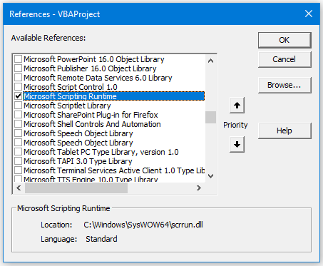
3. - कोड डालने के बाद क्लिक करें टूल्स > संदर्भ खुले में अनुप्रयोगों के लिए माइक्रोसॉफ्ट विज़ुअल बेसिक विंडो, और फिर, पॉप आउट में सन्दर्भ - वीबीएप्रोजेक्ट संवाद बॉक्स, जाँचें माइक्रोसॉफ्ट स्क्रिप्टिंग रनटाइम में विकल्प उपलब्ध संदर्भ सूची बॉक्स, स्क्रीनशॉट देखें:
 |
 |
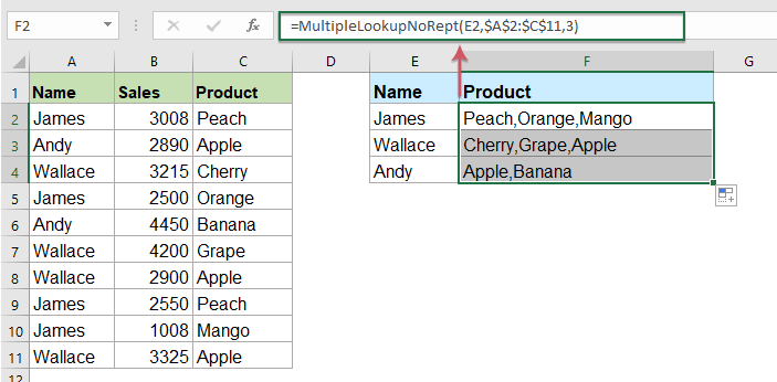
4। तब दबायें OK संवाद बॉक्स को बंद करने के लिए, कोड विंडो को सहेजें और बंद करें, वर्कशीट पर वापस लौटें और इस सूत्र को दर्ज करें: =MultipleLookupNoRept(E2,$A$2:$C$11,3) into a blank cell where you want to output the result, and then drag the fill hanlde down to get all matching values, see screenshot:
एक उपयोगी सुविधा के साथ एक सेल में एकाधिक मान लौटाने के लिए Vlookup
यदि आपके पास हमारा एक्सेल के लिए कुटूल, के साथ अपने उन्नत संयोजन पंक्तियाँ सुविधा, आप समान मान के आधार पर पंक्तियों को शीघ्रता से मर्ज या संयोजित कर सकते हैं और अपनी आवश्यकतानुसार कुछ गणनाएँ कर सकते हैं।
स्थापित करने के बाद एक्सेल के लिए कुटूल, कृपया निम्नानुसार करें:
1. उस डेटा श्रेणी का चयन करें जिसमें आप एक कॉलम डेटा को दूसरे कॉलम के आधार पर संयोजित करना चाहते हैं।
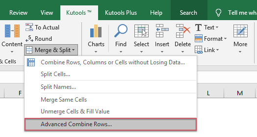
2। क्लिक करें कुटूल > विलय और विभाजन > उन्नत संयोजन पंक्तियाँ, स्क्रीनशॉट देखें:
3. बाहर निकले में उन्नत संयोजन पंक्तियाँ संवाद बकस:
- जिस कुंजी कॉलम नाम के आधार पर संयोजन करना है उस पर क्लिक करें और फिर क्लिक करें प्राथमिक कुंजी
- फिर दूसरे कॉलम पर क्लिक करें जिसके डेटा को आप कुंजी कॉलम के आधार पर संयोजित करना चाहते हैं और क्लिक करें मिलाना संयुक्त डेटा को अलग करने के लिए एक विभाजक चुनना।
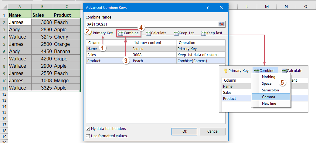
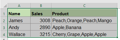
4. तब क्लिक करो OK बटन, और आपको निम्नलिखित परिणाम मिलेंगे:
 |
 |
एक्सेल के लिए कुटूल अभी डाउनलोड करें और निःशुल्क परीक्षण करें!
अधिक संबंधित लेख:
- कुछ बुनियादी और उन्नत उदाहरणों के साथ VLOOKUP फ़ंक्शन
- Excel में, VLOOKUP फ़ंक्शन अधिकांश Excel उपयोगकर्ताओं के लिए एक शक्तिशाली फ़ंक्शन है, जिसका उपयोग डेटा रेंज के सबसे बाईं ओर एक मान को देखने के लिए किया जाता है, और आपके द्वारा निर्दिष्ट कॉलम से उसी पंक्ति में एक मिलान मान लौटाता है। यह ट्यूटोरियल Excel में कुछ बुनियादी और उन्नत उदाहरणों के साथ VLOOKUP फ़ंक्शन का उपयोग करने के तरीके के बारे में बात कर रहा है।
- एक या एकाधिक मानदंडों के आधार पर एकाधिक मिलान मान लौटाएं
- आम तौर पर, VLOOKUP फ़ंक्शन का उपयोग करके हममें से अधिकांश के लिए एक विशिष्ट मान खोजना और मिलान आइटम वापस करना आसान होता है। लेकिन, क्या आपने कभी एक या अधिक मानदंडों के आधार पर एकाधिक मिलान मान वापस करने का प्रयास किया है? इस लेख में, मैं एक्सेल में इस जटिल कार्य को हल करने के लिए कुछ सूत्र पेश करूंगा।
- Vlookup और एकाधिक मानों को लंबवत रूप से लौटाएँ
- आम तौर पर, आप पहला संगत मान प्राप्त करने के लिए Vlookup फ़ंक्शन का उपयोग कर सकते हैं, लेकिन, कभी-कभी, आप एक विशिष्ट मानदंड के आधार पर सभी मिलान रिकॉर्ड वापस करना चाहते हैं। इस लेख में, मैं इस बारे में बात करूंगा कि कैसे सभी मिलान मानों को लंबवत, क्षैतिज या एक ही सेल में वापस लाया जाए।
- Vlookup और ड्रॉप डाउन सूची से एकाधिक मान लौटाएँ
- एक्सेल में, आप ड्रॉप डाउन सूची से कई संबंधित मानों को कैसे देख सकते हैं और वापस कर सकते हैं, जिसका अर्थ है कि जब आप ड्रॉप डाउन सूची से एक आइटम चुनते हैं, तो उसके सभी संबंधित मान एक ही बार में प्रदर्शित होते हैं। इस लेख में, मैं चरण दर चरण समाधान पेश करूंगा।
सर्वोत्तम कार्यालय उत्पादकता उपकरण
एक्सेल के लिए कुटूल के साथ अपने एक्सेल कौशल को सुपरचार्ज करें, और पहले जैसी दक्षता का अनुभव करें। एक्सेल के लिए कुटूल उत्पादकता बढ़ाने और समय बचाने के लिए 300 से अधिक उन्नत सुविधाएँ प्रदान करता है। वह सुविधा प्राप्त करने के लिए यहां क्लिक करें जिसकी आपको सबसे अधिक आवश्यकता है...
")
ऑफिस टैब ऑफिस में टैब्ड इंटरफ़ेस लाता है, और आपके काम को बहुत आसान बनाता है
- Word, Excel, PowerPoint में टैब्ड संपादन और रीडिंग सक्षम करें, प्रकाशक, एक्सेस, विसियो और प्रोजेक्ट।
- नई विंडो के बजाय एक ही विंडो के नए टैब में एकाधिक दस्तावेज़ खोलें और बनाएं।
- आपकी उत्पादकता 50% बढ़ जाती है, और आपके लिए हर दिन सैकड़ों माउस क्लिक कम हो जाते हैं!
")