एक्सेल में एकाधिक कॉलम से अद्वितीय मान कैसे निकालें?
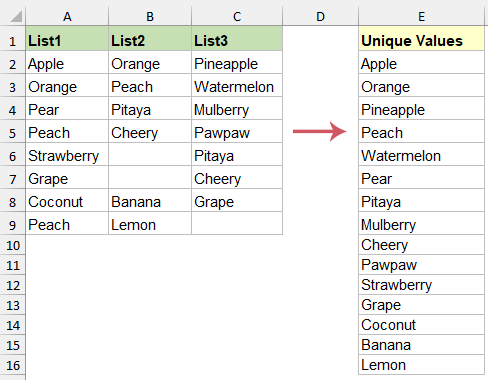
मान लीजिए कि आपके पास एकाधिक मानों वाले कई कॉलम हैं, तो कुछ मान एक ही कॉलम या अलग-अलग कॉलम में दोहराए जाते हैं। और अब आप उन मानों को ढूंढना चाहते हैं जो किसी भी कॉलम में केवल एक बार मौजूद हैं। क्या एक्सेल में एकाधिक कॉलम से अद्वितीय मान निकालने के लिए आपके पास कोई त्वरित तरकीबें हैं?
सूत्रों के साथ एकाधिक स्तंभों से अद्वितीय मान निकालें
यह अनुभाग दो सूत्रों को कवर करेगा: एक सभी एक्सेल संस्करणों के लिए उपयुक्त सरणी सूत्र का उपयोग करना, और दूसरा एक्सेल 365 के लिए विशेष रूप से गतिशील सरणी सूत्र का उपयोग करना।
सभी एक्सेल संस्करणों के लिए ऐरे फॉर्मूला के साथ एकाधिक कॉलम से अद्वितीय मान निकालें
एक्सेल के किसी भी संस्करण वाले उपयोगकर्ताओं के लिए, सरणी सूत्र कई कॉलमों में अद्वितीय मान निकालने के लिए एक शक्तिशाली उपकरण हो सकते हैं। यहां बताया गया है कि आप यह कैसे कर सकते हैं:
1. अपने मूल्यों को सीमा में मानकर ए 2: सी 9, कृपया सेल E2 में निम्नलिखित सूत्र दर्ज करें:
=INDIRECT(TEXT(MIN(IF(($A$2:$C$9<>"")*(COUNTIF($E$1:E1,$A$2:$C$9)=0),ROW($2:$9)*100+COLUMN($A:$C),7^8)),"R0C00"),)&""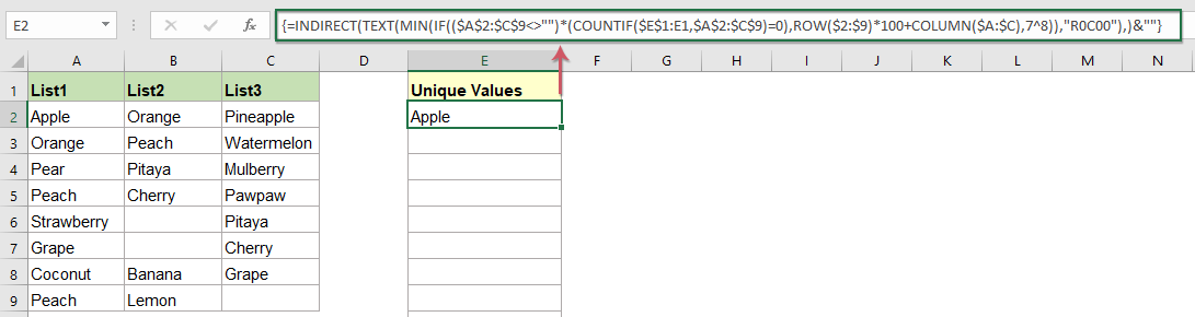
2। फिर दबायें शिफ्ट + Ctrl + एंटर कुंजियाँ एक साथ, और फिर रिक्त कक्ष दिखाई देने तक अद्वितीय मान निकालने के लिए भरण हैंडल को खींचें। स्क्रीनशॉट देखें:

- $ए$2:$सी$9: यह जांचे जाने वाले डेटा रेंज को निर्दिष्ट करता है, जो A2 से C9 तक की कोशिकाएं हैं।
- IF(($A$2:$C$9<>"")*(COUNTIF($E$1:E1,$A$2:$C$9)=0), ROW($2:$9)*100+COLUMN($A:$C), 7^8):
- $A$2:$C$9<>"" जाँचता है कि श्रेणी में कोशिकाएँ खाली तो नहीं हैं।
- COUNTIF($E$1:E1,$A$2:$C$9)=0 यह निर्धारित करता है कि क्या इन कोशिकाओं के मान अभी तक E1 से E1 तक की कोशिकाओं की श्रेणी में सूचीबद्ध नहीं किए गए हैं।
- यदि दोनों शर्तें पूरी होती हैं (यानी, मान खाली नहीं है और अभी तक कॉलम ई में सूचीबद्ध नहीं है), IF फ़ंक्शन अपनी पंक्ति और कॉलम के आधार पर एक अद्वितीय संख्या की गणना करता है (ROW($2:$9)*100+COLUMN($A: $सी)).
- यदि शर्तें पूरी नहीं होती हैं, तो फ़ंक्शन एक बड़ी संख्या (7^8) लौटाता है, जो प्लेसहोल्डर के रूप में कार्य करता है।
- न्यूनतम(...): अगले अद्वितीय मान के स्थान के अनुरूप, उपरोक्त IF फ़ंक्शन द्वारा लौटाई गई सबसे छोटी संख्या ढूँढता है।
- पाठ(...,"R0C00"): इस न्यूनतम संख्या को R1C1 शैली पते में परिवर्तित करता है। प्रारूप कोड R0C00 संख्या के एक्सेल सेल संदर्भ प्रारूप में रूपांतरण को इंगित करता है।
- अप्रत्यक्ष(...): पिछले चरण में उत्पन्न R1C1 शैली पते को सामान्य A1 शैली सेल संदर्भ में परिवर्तित करने के लिए अप्रत्यक्ष फ़ंक्शन का उपयोग करता है। अप्रत्यक्ष फ़ंक्शन टेक्स्ट स्ट्रिंग की सामग्री के आधार पर सेल संदर्भ की अनुमति देता है।
- &"": सूत्र के अंत में &"" जोड़ने से यह सुनिश्चित होता है कि अंतिम आउटपुट को टेक्स्ट के रूप में माना जाएगा, इसलिए सम संख्याओं को टेक्स्ट के रूप में प्रदर्शित किया जाएगा।
Excel 365 के फ़ॉर्मूले के साथ एकाधिक स्तंभों से अद्वितीय मान निकालें
Excel 365 गतिशील सरणियों का समर्थन करता है, जिससे एकाधिक स्तंभों से अद्वितीय मान निकालना बहुत आसान हो जाता है:
कृपया निम्नलिखित सूत्र को एक रिक्त कक्ष में दर्ज करें या कॉपी करें जहां आप परिणाम डालना चाहते हैं, और फिर क्लिक करें दर्ज सभी अद्वितीय मान एक साथ प्राप्त करने की कुंजी। स्क्रीनशॉट देखें:
=UNIQUE(TOCOL(A2:C9,1))
Kutools AI Aide के साथ अनेक स्तंभों से अद्वितीय मान निकालें
की शक्ति को उजागर करें कुटूल्स एआई सहयोगी एक्सेल में एकाधिक कॉलम से अद्वितीय मानों को निर्बाध रूप से निकालने के लिए। बस कुछ ही क्लिक के साथ, यह बुद्धिमान उपकरण आपके डेटा को छानता है, किसी भी चयनित सीमा में अद्वितीय प्रविष्टियों की पहचान करता है और सूचीबद्ध करता है। जटिल फ़ॉर्मूले या वीबीए कोड की परेशानी को भूल जाइए; की दक्षता को अपनाइए कुटूल्स एआई सहयोगी और अपने एक्सेल वर्कफ़्लो को अधिक उत्पादक और त्रुटि-मुक्त अनुभव में बदलें।
एक्सेल के लिए कुटूल इंस्टॉल करने के बाद कृपया क्लिक करें कुटूल्स एआई > ऐ सहयोगी को खोलने के लिए कुटूल्स एआई सहयोगी फलक:
- चैट बॉक्स में अपनी आवश्यकता टाइप करें और क्लिक करें भेजें
बटन या प्रेस दर्ज प्रश्न भेजने की कुंजी;
"रिक्त कक्षों को अनदेखा करते हुए, श्रेणी A2:C9 से अद्वितीय मान निकालें, और परिणामों को E2 से शुरू करें:" - विश्लेषण करने के बाद क्लिक करें निष्पादित करना चलाने के लिए बटन. कुटूल्स एआई सहयोगी एआई का उपयोग करके आपके अनुरोध को संसाधित करेगा और परिणाम सीधे एक्सेल में निर्दिष्ट सेल में लौटाएगा।

पिवट टेबल के साथ एकाधिक कॉलम से अद्वितीय मान निकालें
यदि आप पिवट टेबल से परिचित हैं, तो आप निम्नलिखित चरणों के साथ कई कॉलमों से अद्वितीय मान आसानी से निकाल सकते हैं:
1. सबसे पहले, कृपया अपने डेटा के बाईं ओर एक नया रिक्त कॉलम डालें, इस उदाहरण में, मैं मूल डेटा के बगल में कॉलम ए डालूंगा।

2. अपने डेटा में एक सेल पर क्लिक करें और दबाएँ Alt + D कुंजियाँ, फिर दबाएँ P खोलने के लिए तुरंत कुंजी पिवट टेबल और पिवट चार्ट विजार्ड, चुनें एकाधिक समेकन श्रेणियाँ विज़ार्ड चरण 1 में, स्क्रीनशॉट देखें:

3। तब दबायें अगला बटन, जांचें मेरे लिए एक पेज फ़ील्ड बनाएं विज़ार्ड चरण 2 में विकल्प, स्क्रीनशॉट देखें:

4. क्लिक करते जाइये अगला बटन, डेटा श्रेणी का चयन करने के लिए क्लिक करें जिसमें कक्षों का बायां नया कॉलम शामिल है, फिर क्लिक करें डेटा श्रेणी को जोड़ने के लिए बटन सभी पर्वतमाला सूची बॉक्स, स्क्रीनशॉट देखें:

5. डेटा रेंज का चयन करने के बाद जारी रखें पर क्लिक करें अगला, विज़ार्ड चरण 3 में, अपनी पसंद के अनुसार चुनें कि आप PivotTable रिपोर्ट कहाँ रखना चाहते हैं।

6. अंत में, क्लिक करें अंत विज़ार्ड को पूरा करने के लिए, और वर्तमान वर्कशीट में एक पिवट टेबल बनाई गई है, फिर सभी फ़ील्ड को अनचेक करें रिपोर्ट में जोड़ने के लिए फ़ील्ड चुनें अनुभाग, स्क्रीनशॉट देखें:

7. फिर फ़ील्ड की जाँच करें वैल्यू या मान को खींचें पंक्तियाँ लेबल, अब आपको एकाधिक कॉलम से अद्वितीय मान इस प्रकार मिलेंगे:

VBA कोड के साथ एकाधिक स्तंभों से अद्वितीय मान निकालें
निम्नलिखित वीबीए कोड के साथ, आप एकाधिक कॉलम से अद्वितीय मान भी निकाल सकते हैं।
1. दबाए रखें ALT + F11 कुंजियाँ, और यह खुल जाती है एप्लीकेशन विंडो के लिए माइक्रोसॉफ्ट विज़ुअल बेसिक.
2। क्लिक करें सम्मिलित करें > मॉड्यूल, और मॉड्यूल विंडो में निम्नलिखित कोड पेस्ट करें।
वीबीए: एकाधिक स्तंभों से अद्वितीय मान निकालें
Sub Uniquedata()
'Updateby Extendoffice
Dim rng As Range
Dim InputRng As Range, OutRng As Range
Set dt = CreateObject("Scripting.Dictionary")
xTitleId = "KutoolsforExcel"
Set InputRng = Application.Selection
Set InputRng = Application.InputBox("Range :", xTitleId, InputRng.Address, Type:=8)
Set OutRng = Application.InputBox("Out put to (single cell):", xTitleId, Type:=8)
For Each rng In InputRng
    If rng.Value <> "" Then
        dt(rng.Value) = ""
    End If
Next
OutRng.Range("A1").Resize(dt.Count) = Application.WorksheetFunction.Transpose(dt.Keys)
End Sub
3। फिर दबायें F5 इस कोड को चलाने के लिए, और एक प्रॉम्प्ट बॉक्स आपको यह याद दिलाने के लिए पॉप अप होगा कि आप उस डेटा रेंज का चयन करें जिसका आप उपयोग करना चाहते हैं। स्क्रीनशॉट देखें:

4। और फिर क्लिक करें OK, एक और प्रॉम्प्ट बॉक्स दिखाई देगा जिससे आप परिणाम डालने के लिए स्थान चुन सकेंगे, स्क्रीनशॉट देखें:

5. क्लिक करें OK इस संवाद को बंद करने के लिए, और सभी अद्वितीय मान एक ही बार में निकाले गए हैं।

अधिक संबंधित लेख:
- किसी सूची से अद्वितीय और विशिष्ट मानों की संख्या गिनें
- मान लीजिए, आपके पास कुछ डुप्लिकेट आइटमों के साथ मानों की एक लंबी सूची है, अब, आप अद्वितीय मानों की संख्या की गणना करना चाहते हैं (वे मान जो सूची में केवल एक बार दिखाई देते हैं) या विशिष्ट मान (सूची में सभी अलग-अलग मान, इसका मतलब अद्वितीय है) मान +पहला डुप्लिकेट मान) एक कॉलम में जैसा कि बाएं स्क्रीनशॉट में दिखाया गया है। इस लेख में, मैं एक्सेल में इस काम से निपटने के तरीके के बारे में बात करूंगा।
- एक्सेल में मानदंड के आधार पर अद्वितीय मान निकालें
- मान लीजिए, आपके पास निम्नलिखित डेटा रेंज है जिसमें आप नीचे दिखाए गए स्क्रीनशॉट के अनुसार परिणाम प्राप्त करने के लिए कॉलम ए के विशिष्ट मानदंड के आधार पर केवल कॉलम बी के अद्वितीय नामों को सूचीबद्ध करना चाहते हैं। आप एक्सेल में इस कार्य को जल्दी और आसानी से कैसे निपटा सकते हैं?
- एक्सेल में केवल अद्वितीय मानों की अनुमति दें
- यदि आप वर्कशीट के कॉलम में केवल अद्वितीय मान दर्ज करना चाहते हैं और डुप्लिकेट को रोकना चाहते हैं, तो यह आलेख इस कार्य से निपटने के लिए आपके लिए कुछ त्वरित युक्तियां पेश करेगा।
- एक्सेल में मानदंड के आधार पर अद्वितीय मानों का योग
- उदाहरण के लिए, मेरे पास डेटा की एक श्रृंखला है जिसमें नाम और ऑर्डर कॉलम शामिल हैं, अब, नाम कॉलम के आधार पर ऑर्डर कॉलम में केवल अद्वितीय मानों को जोड़ने के लिए जैसा कि निम्नलिखित स्क्रीनशॉट में दिखाया गया है। एक्सेल में इस कार्य को जल्दी और आसानी से कैसे हल करें?
सर्वोत्तम कार्यालय उत्पादकता उपकरण
एक्सेल के लिए कुटूल के साथ अपने एक्सेल कौशल को सुपरचार्ज करें, और पहले जैसी दक्षता का अनुभव करें। एक्सेल के लिए कुटूल उत्पादकता बढ़ाने और समय बचाने के लिए 300 से अधिक उन्नत सुविधाएँ प्रदान करता है। वह सुविधा प्राप्त करने के लिए यहां क्लिक करें जिसकी आपको सबसे अधिक आवश्यकता है...
")
ऑफिस टैब ऑफिस में टैब्ड इंटरफ़ेस लाता है, और आपके काम को बहुत आसान बनाता है
- Word, Excel, PowerPoint में टैब्ड संपादन और रीडिंग सक्षम करें, प्रकाशक, एक्सेस, विसियो और प्रोजेक्ट।
- नई विंडो के बजाय एक ही विंडो के नए टैब में एकाधिक दस्तावेज़ खोलें और बनाएं।
- आपकी उत्पादकता 50% बढ़ जाती है, और आपके लिए हर दिन सैकड़ों माउस क्लिक कम हो जाते हैं!
")