मुख्य सामग्री पर जाएं

एक्सेल में मानदंड के आधार पर अद्वितीय मान कैसे निकालें?

लेखक: ज़ियाओयांग अंतिम संशोधित: 2021-10-22

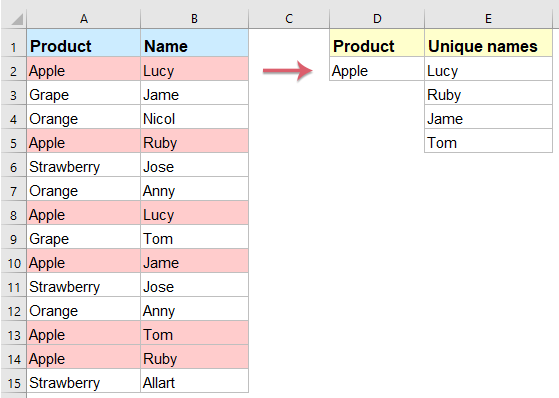
मान लीजिए, आपके पास बाईं डेटा श्रेणी है जिसमें आप नीचे दिखाए गए स्क्रीनशॉट के अनुसार परिणाम प्राप्त करने के लिए कॉलम ए के विशिष्ट मानदंड के आधार पर केवल कॉलम बी के अद्वितीय नामों को सूचीबद्ध करना चाहते हैं। आप एक्सेल में इस कार्य को जल्दी और आसानी से कैसे निपटा सकते हैं?

सरणी सूत्र के साथ मानदंड के आधार पर अद्वितीय मान निकालें

सरणी सूत्र के साथ अनेक मानदंडों के आधार पर अद्वितीय मान निकालें

किसी उपयोगी सुविधा के साथ कक्षों की सूची से अद्वितीय मान निकालें


सरणी सूत्र के साथ मानदंड के आधार पर अद्वितीय मान निकालें

इस कार्य को हल करने के लिए, आप एक जटिल सरणी सूत्र लागू कर सकते हैं, कृपया निम्नानुसार कार्य करें:

1. नीचे दिए गए सूत्र को एक रिक्त सेल में दर्ज करें जहां आप निकाले गए परिणाम को सूचीबद्ध करना चाहते हैं, इस उदाहरण में, मैं इसे सेल E2 में रखूंगा, और फिर दबाऊंगा शिफ्ट + Ctrl + एंटर पहला अद्वितीय मान प्राप्त करने के लिए कुंजियाँ।

=IFERROR(INDEX($B$2:$B$15, MATCH(0, IF($D$2=$A$2:$A$15, COUNTIF($E$1:$E1, $B$2:$B$15), ""), 0)),"")

2. फिर, रिक्त सेल प्रदर्शित होने तक भरण हैंडल को नीचे की ओर खींचें, और अब विशिष्ट मानदंड के आधार पर सभी अद्वितीय मान सूचीबद्ध किए गए हैं, स्क्रीनशॉट देखें:

नोट: उपरोक्त सूत्र में: B2: B15 क्या स्तंभ श्रेणी में वे अद्वितीय मान शामिल हैं जिन्हें आप निकालना चाहते हैं, A2: A15 क्या कॉलम में वह मानदंड शामिल है जिसके आधार पर आप हैं, D2 उस मानदंड को इंगित करता है जिसके आधार पर आप अद्वितीय मानों को सूचीबद्ध करना चाहते हैं, और E1 आपके दर्ज किए गए फ़ॉर्मूले के ऊपर की सेल है.

सरणी सूत्र के साथ अनेक मानदंडों के आधार पर अद्वितीय मान निकालें

यदि आप दो स्थितियों के आधार पर अद्वितीय मान निकालना चाहते हैं, तो यहां एक और सरणी सूत्र है जो आपकी मदद कर सकता है, कृपया इसे इस प्रकार करें:

1. नीचे दिए गए सूत्र को एक रिक्त कक्ष में दर्ज करें जहां आप अद्वितीय मानों को सूचीबद्ध करना चाहते हैं, इस उदाहरण में, मैं इसे कक्ष G2 में रखूंगा, और फिर दबाऊंगा शिफ्ट + Ctrl + एंटर पहला अद्वितीय मान प्राप्त करने के लिए कुंजियाँ।

=IFERROR(INDEX($C$2:$C$15,MATCH(0,COUNTIF(G1:$G$1,$C$2:$C$15)+IF($A$2:$A$15<>$E$2,1,0)+IF($B$2:$B$15<>$F$2,1,0),0)),"")

2. फिर, रिक्त कक्ष प्रदर्शित होने तक भरण हैंडल को कक्षों तक नीचे खींचें, और अब विशिष्ट दो स्थितियों के आधार पर सभी अद्वितीय मान सूचीबद्ध किए गए हैं, स्क्रीनशॉट देखें:

नोट: उपरोक्त सूत्र में: सी2:सी15 क्या स्तंभ श्रेणी में वे अद्वितीय मान शामिल हैं जिन्हें आप निकालना चाहते हैं, A2: A15 और E2 मानदंड वाली पहली श्रेणी है जिसके आधार पर आप अद्वितीय मान निकालना चाहते हैं, B2: B15 और F2 मानदंड के साथ दूसरी श्रेणी है जिसके आधार पर आप अद्वितीय मान निकालना चाहते हैं, और G1 आपके दर्ज किए गए फ़ॉर्मूले के ऊपर की सेल है.

किसी उपयोगी सुविधा के साथ कक्षों की सूची से अद्वितीय मान निकालें

कभी-कभी, आप केवल कोशिकाओं की सूची से अद्वितीय मान निकालना चाहते हैं, यहां, मैं एक उपयोगी टूल की सिफारिश करूंगा-एक्सेल के लिए कुटूल, के साथ अपने अद्वितीय मान वाले सेल निकालें (पहला डुप्लिकेट शामिल करें) उपयोगिता, आप तुरंत अद्वितीय मान निकाल सकते हैं।

नोट:इसे लागू करने के लिए अद्वितीय मान वाले सेल निकालें (पहला डुप्लिकेट शामिल करें), सबसे पहले, आपको डाउनलोड करना चाहिए एक्सेल के लिए कुटूल, और फिर सुविधा को जल्दी और आसानी से लागू करें।

स्थापित करने के बाद एक्सेल के लिए कुटूल, कृपया ऐसा करें:

1. उस सेल पर क्लिक करें जहां आप परिणाम आउटपुट करना चाहते हैं। (नोट:पहली पंक्ति में किसी सेल पर क्लिक न करें.)

2। तब दबायें कुटूल > फॉर्मूला हेल्पर > फॉर्मूला हेल्पर, स्क्रीनशॉट देखें:

3. में सूत्र सहायक संवाद बॉक्स, कृपया निम्नलिखित कार्य करें:

  • चुनते हैं टेक्स्ट से विकल्प सूत्र प्रकार ड्रॉप डाउन सूची;
  • उसके बाद चुनो अद्वितीय मान वाले सेल निकालें (पहला डुप्लिकेट शामिल करें) से एक फ्रोमुला चुनें सूची बाक्स;
  • सही तर्क इनपुट अनुभाग में, उन कक्षों की सूची चुनें जिनसे आप अद्वितीय मान निकालना चाहते हैं।

4। तब दबायें Ok बटन, पहला परिणाम सेल में प्रदर्शित होता है, फिर सेल का चयन करें और भरण हैंडल को उन सेल पर खींचें जिनमें आप सभी अद्वितीय मानों को सूचीबद्ध करना चाहते हैं जब तक कि रिक्त सेल दिखाई न दें, स्क्रीनशॉट देखें:

एक्सेल के लिए अभी नि:शुल्क कुटूल डाउनलोड करें!


अधिक संबंधित लेख:

  • किसी सूची से अद्वितीय और विशिष्ट मानों की संख्या गिनें
  • मान लीजिए, आपके पास कुछ डुप्लिकेट आइटमों के साथ मानों की एक लंबी सूची है, अब, आप अद्वितीय मानों की संख्या की गणना करना चाहते हैं (वे मान जो सूची में केवल एक बार दिखाई देते हैं) या विशिष्ट मान (सूची में सभी अलग-अलग मान, इसका मतलब अद्वितीय है) मान +पहला डुप्लिकेट मान) एक कॉलम में जैसा कि बाएं स्क्रीनशॉट में दिखाया गया है। इस लेख में, मैं एक्सेल में इस काम से निपटने के तरीके के बारे में बात करूंगा।
  • एक्सेल में मानदंड के आधार पर अद्वितीय मानों का योग
  • उदाहरण के लिए, मेरे पास डेटा की एक श्रृंखला है जिसमें नाम और ऑर्डर कॉलम शामिल हैं, अब, नाम कॉलम के आधार पर ऑर्डर कॉलम में केवल अद्वितीय मानों को जोड़ने के लिए जैसा कि निम्नलिखित स्क्रीनशॉट में दिखाया गया है। एक्सेल में इस कार्य को जल्दी और आसानी से कैसे हल करें?
  • एक्सेल में अद्वितीय मानों को संयोजित करें
  • यदि मेरे पास मानों की एक लंबी सूची है जो कुछ डुप्लिकेट डेटा से भरी हुई है, तो अब, मैं केवल अद्वितीय मान ढूंढना चाहता हूं और फिर उन्हें एक ही सेल में जोड़ना चाहता हूं। मैं Excel में इस समस्या से शीघ्रता और आसानी से कैसे निपट सकता हूँ?

सर्वोत्तम कार्यालय उत्पादकता उपकरण

🤖 कुटूल्स एआई सहयोगी: निम्न के आधार पर डेटा विश्लेषण में क्रांति लाएं: बुद्धिमान निष्पादन   |  कोड जनरेट करें  |  कस्टम फ़ॉर्मूले बनाएं  |  डेटा का विश्लेषण करें और चार्ट बनाएं  |  कुटूल फ़ंक्शंस का आह्वान करें...
लोकप्रिय सुविधाएँ: डुप्लिकेट ढूंढें, हाइलाइट करें या पहचानें   |  रिक्त पंक्तियाँ हटाएँ   |  डेटा खोए बिना कॉलम या सेल को संयोजित करें   |   फॉर्मूला के बिना गोल ...
सुपर लुकअप: एकाधिक मानदंड VLookup    मल्टीपल वैल्यू वीलुकअप  |   अनेक शीटों में VLookup   |   फजी लुकअप ....
उन्नत ड्रॉप-डाउन सूची: शीघ्रता से ड्रॉप डाउन सूची बनाएं   |  आश्रित ड्रॉप डाउन सूची   |  बहु-चयन ड्रॉप डाउन सूची ....
स्तम्भ प्रबंधक: कॉलमों की एक विशिष्ट संख्या जोड़ें  |  कॉलम ले जाएँ  |  छिपे हुए कॉलम की दृश्यता स्थिति टॉगल करें  |  रेंज और कॉलम की तुलना करें ...
फीचर्ड फीचर्स: ग्रिड फोकस   |  डिजाइन देखें   |   बड़ा फॉर्मूला बार    कार्यपुस्तिका एवं शीट प्रबंधक   |  संसाधन लाइब्रेरी (ऑटो टेक्स्ट)   |  खजूर बीनने वाला   |  कार्यपत्रकों को संयोजित करें   |  एन्क्रिप्ट/डिक्रिप्ट सेल    सूची के अनुसार ईमेल भेजें   |  सुपर फ़िल्टर   |   विशेष फ़िल्टर (फ़िल्टर बोल्ड/इटैलिक/स्ट्राइकथ्रू...) ...
शीर्ष 15 टूलसेट12 टेक्स्ट टूल्स (पाठ जोड़ें, अक्षर हटाएँ, ...)   |   50 + चार्ट प्रकार (गैन्ट चार्ट, ...)   |   40+ प्रैक्टिकल सूत्र (जन्मदिन के आधार पर आयु की गणना करें, ...)   |   19 निवेशन टूल्स (QR कोड डालें, पथ से चित्र सम्मिलित करें, ...)   |   12 रूपांतरण टूल्स (शब्दों को संख्याएँ, मुद्रा रूपांतरण, ...)   |   7 विलय और विभाजन टूल्स (उन्नत संयोजन पंक्तियाँ, विभाजन कोशिकाओं, ...)   |   ... और अधिक

एक्सेल के लिए कुटूल के साथ अपने एक्सेल कौशल को सुपरचार्ज करें, और पहले जैसी दक्षता का अनुभव करें। एक्सेल के लिए कुटूल उत्पादकता बढ़ाने और समय बचाने के लिए 300 से अधिक उन्नत सुविधाएँ प्रदान करता है।  वह सुविधा प्राप्त करने के लिए यहां क्लिक करें जिसकी आपको सबसे अधिक आवश्यकता है...

Description


ऑफिस टैब ऑफिस में टैब्ड इंटरफ़ेस लाता है, और आपके काम को बहुत आसान बनाता है

  • Word, Excel, PowerPoint में टैब्ड संपादन और रीडिंग सक्षम करें, प्रकाशक, एक्सेस, विसियो और प्रोजेक्ट।
  • नई विंडो के बजाय एक ही विंडो के नए टैब में एकाधिक दस्तावेज़ खोलें और बनाएं।
  • आपकी उत्पादकता 50% बढ़ जाती है, और आपके लिए हर दिन सैकड़ों माउस क्लिक कम हो जाते हैं!
Comments (40)
No ratings yet. Be the first to rate!
This comment was minimized by the moderator on the site
Thank you so much. This was very very helpful. You Rock!!
This comment was minimized by the moderator on the site
hi everyone..
i have problem..
i got blank result even i press ctrl shift enter together..
This comment was minimized by the moderator on the site
Hi all, Can some help me to get all unique values on one single cell
This comment was minimized by the moderator on the site
Hi, this worked well! Although it takes Excel sooooo long to calculate. Just dragging down 15 cells in a column takes about 15min to calculate... if not longer. Is this normal? If this becomes dynamic it will take a hell of alot of computing time.
This comment was minimized by the moderator on the site
Hello. This is really helpful, however, what If I want a formula that lists the unique values based on multiple criteria. eg. I have a data set which has the following data in a table (after each hyphen is a new column but same row):

Company A - £200 - £100
Company A - £300 - £200
Company B - £300 - £200
Company C - £600 - £200
Company B - £100 - £300
Company D - £0 - £600
Company A - £700 - £100

I want a new data table in a new tab which groups the duplicate values without using an array formula. currently I'm grouping using a pivot table and pasting to my new data table. It's a long process but array formulas make my spreadsheet really slow.

Company A - £1200 - £400
Company B - £400 - £500
Company C - £600 - £200
Company D - £0 - £600

Thanks,
K
This comment was minimized by the moderator on the site
Hello, K,
For solving your problem, I can recommend our useful tool- Kutools for Excel, with its Advanced Combine Rows feature, you can deal with this job quickly. Firstly, you should copy and paste your data into a new worksheet, and then apply htis feature as below screenhsot shown.
You can know more about this feature from: https://www.extendoffice.com/product/kutools-for-excel/excel-combine-duplicate-rows.html
Please download Kutools for Excel and install it, then apply this feature. Full feature free trial 30-day, please try.
This comment was minimized by the moderator on the site
Hi! the formula works really well. I would like to add another criterion, i mean, get the unique answers but using two criteria
This comment was minimized by the moderator on the site
Hi, Giancarlo,
to extract unique values based on multiple criteria, any of the below formula can help you: (after pasting the formula, please press Ctrl + Shift + Enter keys together.)
=IFERROR(INDEX($C$2:$C$11, MATCH(0, COUNTIF(G1:$G$1, $C$2:$C$11)+IF($A$2:$A$11<>$E$2, 1, 0)+IF($B$2:$B$11<>$F$2, 1, 0), 0)), "")
=INDEX($C$2:$C$11, MATCH(0, IF(($A$2:$A$11=$E$2)*($B$2:$B$11=$F$2), COUNTIF($G$1:$G1, $C$2:$C$11), ""), 0))
Please try, hope it can help you!
This comment was minimized by the moderator on the site
Hi. I am using the two conditions formula =IFERROR(INDEX($C$2:$C$11, MATCH(0, COUNTIF(G1:$G$1, $C$2:$C$11)+IF($A$2:$A$11<>$E$2, 1, 0)+IF($B$2:$B$11<>$F$2, 1, 0), 0)), "") to extract a unique list and it works great, but I am struggle to add the SMALL function to get the list sorted as well in ascending order. Are you able to help?
This comment was minimized by the moderator on the site
Is there a way to make this work while ALLOWING for duplicate values? For instance, I want all instances of Lucy to be listed in the results.
This comment was minimized by the moderator on the site
Hello, Konstantin,
To extract all corresponding values including the duplicates based on a specific cell criteria, the following array formula can help you, see screenshot:
=IF(ISERROR(INDEX($A$1:$B$17,SMALL(IF($A$1:$A$17=$D$2,ROW($A$1:$A$17)),ROW(1:1)),2)),"",
INDEX($A$1:$B$17,SMALL(IF($A$1:$A$17=$D$2,ROW($A$1:$A$17)),ROW(1:1)),2))

After inserting the formula, please press Shift + Ctrl + Enter keys together to get the correct result, and then drag the fill handle down to get all values.
Hope this can help you, thank you!
This comment was minimized by the moderator on the site
This has worked great for me with a specific lookup value. However, if I wanted to use a wildcard to look up partial values, how would I do that? For example, if I wanted to lookup all the names associated with KT?

I am using this function to look up cells that contain multiple text. For example if each product also had a sub-product within the same cell but I was only looking for names associated with the sub-product "elf".

KTE - elf
KTE- ball
KTE - piano
KTO - elf
KTO- ball
KTO - piano
This comment was minimized by the moderator on the site
For me the formula does not work. I press ctrl shift enter and i still get an error N/A. I would like to add that i prpared exaclty the same data as in tutorial. What is the reason it does not work?
This comment was minimized by the moderator on the site
How would I get this formula to return each of the duplicates instead of one of each of the names? For instance, in the example above, how would I get the results column (B:B) to return Lucy, Ruby, Anny, Jose, Lucy, Anny, Tom? I'm using this as a budget tool pulling to specific account summaries from a general ledger. However, several of the amounts and transaction descriptions are duplicates in the general ledger. Once the first of the duplicated values is pulled, no more of them get pulled.
This comment was minimized by the moderator on the site
Hi, Joe,
To extract all corresponding values based on a specific cell criteria, the following array formula can help you, see screenshot:
=IF(ISERROR(INDEX($A$1:$B$17,SMALL(IF($A$1:$A$17=$D$2,ROW($A$1:$A$17)),ROW(1:1)),2)),"",
INDEX($A$1:$B$17,SMALL(IF($A$1:$A$17=$D$2,ROW($A$1:$A$17)),ROW(1:1)),2))

After inserting the formula, please press Shift + Ctrl + Enter keys together to get the correct result, and then drag the fill handle down to get all values.
Hope this can help you, thank you!
This comment was minimized by the moderator on the site
Last Question: If I want the results column to return all values not associated with KTE or KTO (so, D:D would be Tom, Nocol, Lily, Angelina, Genna), how would I do that?
This comment was minimized by the moderator on the site
Ok, so it works in the master workbook. There is one exception that I haven't been able to determine the cause of: If the array (in my case, the general ledger that I had beginning in row 3) does not begin in Row 1, the returned values are incorrect. What causes this problem, and which term in the formula fixes it? Thanks again for your help with this!
This comment was minimized by the moderator on the site
So far so good. I'm able to duplicate the results in the test sheet, make changes to the array, and then correct the formula to account for the changes I've made. I plan to move this into the master sheet today and see how it works. Thanks for the help!
There are no comments posted here yet
Load More
Please leave your comments in English
Posting as Guest
×
Rate this post:
0   Characters
Suggested Locations