मुख्य सामग्री पर जाएं

एक्सेल में आज से कम/अधिक तिथियों को सशर्त प्रारूपित कैसे करें?

लेखक: सिलुविया अंतिम संशोधित: 2020-04-23

आप एक्सेल में वर्तमान दिनांक के आधार पर दिनांकों को सशर्त प्रारूपित कर सकते हैं। उदाहरण के लिए, आप आज से पहले की तिथियों को प्रारूपित कर सकते हैं, या आज से बड़ी तिथियों को प्रारूपित कर सकते हैं। इस ट्यूटोरियल में, हम आपको दिखाएंगे कि Excel में देय तिथियों या भविष्य की तिथियों को विस्तार से उजागर करने के लिए सशर्त स्वरूपण में TODAY फ़ंक्शन का उपयोग कैसे करें।

एक्सेल में सशर्त प्रारूप की तारीखें आज से पहले की या भविष्य की तारीखें


एक्सेल में सशर्त प्रारूप की तारीखें आज से पहले की या भविष्य की तारीखें

मान लीजिए कि आपके पास दिनांक की एक सूची है जैसा कि नीचे स्क्रीनशॉट में दिखाया गया है। देय तिथियों और भविष्य की बकाया तिथियों को बकाया करने के लिए कृपया निम्नानुसार कार्य करें।

1. रेंज A2:A15 चुनें, फिर क्लिक करें सशर्त फॉर्मेटिंग > नियम प्रबंधित करें के अंतर्गत होम टैब. स्क्रीनशॉट देखें:

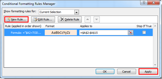
2। में सशर्त स्वरूपण नियम प्रबंधक संवाद बॉक्स में, क्लिक करें नए नियम बटन.

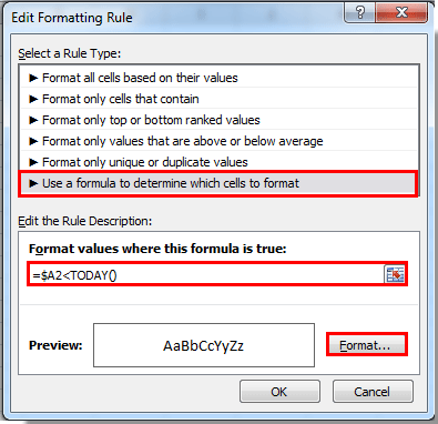
3। में नया प्रारूपण नियम संवाद बॉक्स, आपको यह करना होगा:

1). चुनना नियम प्रकार चुनें में कौन से कक्षों को प्रारूपित करना है यह निर्धारित करने के लिए एक सूत्र का उपयोग करें अनुभाग;

2)। के लिये आज से पुरानी तारीखों को फ़ॉर्मेट करना, कृपया सूत्र को कॉपी और पेस्ट करें =$A2<आज() में उन मानों को प्रारूपित करें जहां यह सूत्र सत्य है डिब्बा;

के लिए भविष्य की तारीखों को प्रारूपित करना, कृपया इस सूत्र का उपयोग करें =$A2>आज();

3). क्लिक करें का गठन बटन। स्क्रीनशॉट देखें:

4। में प्रारूप प्रकोष्ठों संवाद बॉक्स में, नियत तिथियों या भविष्य की तिथियों के लिए प्रारूप निर्दिष्ट करें और फिर क्लिक करें OK बटन.

5. फिर यह वापस लौट आता है सशर्त स्वरूपण नियम प्रबंधक संवाद बकस। और नियत दिनांक स्वरूपण नियम बनाया गया है। यदि आप अभी नियम लागू करना चाहते हैं, तो कृपया क्लिक करें लागू करें बटन.

6. लेकिन यदि आप नियत तिथि नियम और भविष्य तिथि नियम को एक साथ लागू करना चाहते हैं, तो कृपया उपरोक्त चरणों को 2 से 4 तक दोहराकर भविष्य तिथि स्वरूपण सूत्र के साथ एक नया नियम बनाएं।

7. जब यह वापस आता है सशर्त स्वरूपण नियम प्रबंधक डायलॉग बॉक्स फिर से, आप देख सकते हैं कि बॉक्स में दो नियम दिख रहे हैं, कृपया क्लिक करें OK फ़ॉर्मेटिंग प्रारंभ करने के लिए बटन.

फिर आप आज से पुरानी तारीखें देख सकते हैं और आज से बड़ी तारीखें सफलतापूर्वक स्वरूपित हो गई हैं।

चयन में प्रत्येक n पंक्ति को आसानी से सशर्त स्वरूपित करें:

एक्सेल के लिए कुटूल's वैकल्पिक पंक्ति/स्तंभ छायांकन उपयोगिता आपको Excel चयन में प्रत्येक n पंक्ति में आसानी से सशर्त स्वरूपण जोड़ने में मदद करती है।
एक्सेल के लिए कुटूल्स का पूर्ण फीचर 30-दिवसीय निःशुल्क ट्रेल अभी डाउनलोड करें!


संबंधित आलेख:

सर्वोत्तम कार्यालय उत्पादकता उपकरण

🤖 कुटूल्स एआई सहयोगी: निम्न के आधार पर डेटा विश्लेषण में क्रांति लाएं: बुद्धिमान निष्पादन   |  कोड जनरेट करें  |  कस्टम फ़ॉर्मूले बनाएं  |  डेटा का विश्लेषण करें और चार्ट बनाएं  |  कुटूल फ़ंक्शंस का आह्वान करें...
लोकप्रिय सुविधाएँ: डुप्लिकेट ढूंढें, हाइलाइट करें या पहचानें   |  रिक्त पंक्तियाँ हटाएँ   |  डेटा खोए बिना कॉलम या सेल को संयोजित करें   |   फॉर्मूला के बिना गोल ...
सुपर लुकअप: एकाधिक मानदंड VLookup    मल्टीपल वैल्यू वीलुकअप  |   अनेक शीटों में VLookup   |   फजी लुकअप ....
उन्नत ड्रॉप-डाउन सूची: शीघ्रता से ड्रॉप डाउन सूची बनाएं   |  आश्रित ड्रॉप डाउन सूची   |  बहु-चयन ड्रॉप डाउन सूची ....
स्तम्भ प्रबंधक: कॉलमों की एक विशिष्ट संख्या जोड़ें  |  कॉलम ले जाएँ  |  छिपे हुए कॉलम की दृश्यता स्थिति टॉगल करें  |  रेंज और कॉलम की तुलना करें ...
फीचर्ड फीचर्स: ग्रिड फोकस   |  डिजाइन देखें   |   बड़ा फॉर्मूला बार    कार्यपुस्तिका एवं शीट प्रबंधक   |  संसाधन लाइब्रेरी (ऑटो टेक्स्ट)   |  खजूर बीनने वाला   |  कार्यपत्रकों को संयोजित करें   |  एन्क्रिप्ट/डिक्रिप्ट सेल    सूची के अनुसार ईमेल भेजें   |  सुपर फ़िल्टर   |   विशेष फ़िल्टर (फ़िल्टर बोल्ड/इटैलिक/स्ट्राइकथ्रू...) ...
शीर्ष 15 टूलसेट12 टेक्स्ट टूल्स (पाठ जोड़ें, अक्षर हटाएँ, ...)   |   50 + चार्ट प्रकार (गैन्ट चार्ट, ...)   |   40+ प्रैक्टिकल सूत्र (जन्मदिन के आधार पर आयु की गणना करें, ...)   |   19 निवेशन टूल्स (QR कोड डालें, पथ से चित्र सम्मिलित करें, ...)   |   12 रूपांतरण टूल्स (शब्दों को संख्याएँ, मुद्रा रूपांतरण, ...)   |   7 विलय और विभाजन टूल्स (उन्नत संयोजन पंक्तियाँ, विभाजन कोशिकाओं, ...)   |   ... और अधिक

एक्सेल के लिए कुटूल के साथ अपने एक्सेल कौशल को सुपरचार्ज करें, और पहले जैसी दक्षता का अनुभव करें। एक्सेल के लिए कुटूल उत्पादकता बढ़ाने और समय बचाने के लिए 300 से अधिक उन्नत सुविधाएँ प्रदान करता है।  वह सुविधा प्राप्त करने के लिए यहां क्लिक करें जिसकी आपको सबसे अधिक आवश्यकता है...

Description


ऑफिस टैब ऑफिस में टैब्ड इंटरफ़ेस लाता है, और आपके काम को बहुत आसान बनाता है

  • Word, Excel, PowerPoint में टैब्ड संपादन और रीडिंग सक्षम करें, प्रकाशक, एक्सेस, विसियो और प्रोजेक्ट।
  • नई विंडो के बजाय एक ही विंडो के नए टैब में एकाधिक दस्तावेज़ खोलें और बनाएं।
  • आपकी उत्पादकता 50% बढ़ जाती है, और आपके लिए हर दिन सैकड़ों माउस क्लिक कम हो जाते हैं!
Comments (24)
No ratings yet. Be the first to rate!
This comment was minimized by the moderator on the site
I want to highlight a cell if:
1. today's date is greater than the date in another cell or blank (=TODAY()>'APM Tracker'P14) AND ALSO;
2. If the date in P15 is greater than P14 same highlight color AND ALSO;
3. If the date in P15 is less than P14 I do not want the highlight
This comment was minimized by the moderator on the site
Hey All,

I want to get only past due dates in the particular column. Instead of highlighting the cells with color i need the dates to be picked in the column

Any solution for this....
This comment was minimized by the moderator on the site
Alright, I read through this thread and did not see this question asked/answered. I have a column of future dates. I would like to add conditional formatting to flag that date exactly 30 days before (1st color "Hey you should get this done its due in 30 day's") and 7 days ( 2nd color "You procrastinated and now you have 7 days to complete this"). Any help here?
This comment was minimized by the moderator on the site
Hi Michael,
I am not sure I understand your question clearly. If you want to hight the date which is 30 days and 7 days from today. Please use the following formulas to create two formula rules with different highlighted colors:
=D9=TODAY()+30
=D9=TODAY()+7

https://www.extendoffice.com/images/stories/comments/comment-picture-zxm/conditional-formatting.png
If this is not what you need, please attach a screenshot of your data here.
This comment was minimized by the moderator on the site
To ignore cells that have blanks try this:

=AND($A2<>"",$A2<TODAY())

This assumes the cell you have selected is A2 (change this to whatever cell you have currently selected)
To copy this to the applicable cells, change the "Applies to" to the cell range you need.
This comment was minimized by the moderator on the site
Hi Andy Campbell,
Thank you for sharing.
This comment was minimized by the moderator on the site
Hi
I am trying to use condition formatting to allow a cell to be highlighted when an item is past due based on different turn around times (TAT). I have a column with a submitted date which is then used with the #of days from the TAT to automatically give the due date. Using the following formula, =IF(OR(E3="",A3=""),"",DATE(YEAR(A3),MONTH(A3),DAY(A3)+E3))
The condition formatting currently used is "cell value < today()" applies to +$G:$G.
What I would like to do is use the stop if rule to stop the condition formatting if the date entered in column "H" is < or = to todays date.
Thanks Michelle
This comment was minimized by the moderator on the site
if i want highlight the due date with the conditional : today less or equal 30 days from due date
This comment was minimized by the moderator on the site
I am trying to create conditional formatting that will highlight rows older than 14 days in yellow and highlight rows older than 21 days in red. My date column starts in A2, I have the following rules applied, but only yellow is highlighting and just the date column, not the entire row. Can you help? Scott

1. =ISBLANK(A2)=TRUE
2. =A2<TODAY()-14
3. =A2<TODAY()-21
This comment was minimized by the moderator on the site
I want to ignore blank cells which doesn't have a date i.e I do not want blank cells to be highlighted when I am comparing dates<Today(). Please help
This comment was minimized by the moderator on the site
Hi Madhu,
The first method in this artice can help you solve the problem. Please have a try.
https://www.extendoffice.com/documents/excel/2499-excel-conditional-formatting-ignore-blank-zero.html
This comment was minimized by the moderator on the site
1 colum has the dates in it i want another colum to change colour when this formula is applied.

any ideas?
This comment was minimized by the moderator on the site
Hi grant,
Supposing you want to change the cell color in column B based on dates in column A, please select the column B cells (such as B2:B21), and apply the conditional formatting function with the above formulas =$A2>Today() or =$A2<Today().
This comment was minimized by the moderator on the site
Hello! can anyone help me?

I have =TODAY() formula in A1 and need 3 more rules to work as per below

rule 1 all dates 8 to 14 days older than today

rule 2 : all dates older 14 to 30 days than today

rule 3: all dates 31 or more days older than today
This comment was minimized by the moderator on the site
it should be something like this:

if(*cell*+8>Today();if(*cell*+14<Today();"8-14 from today";"N/A"))
There are no comments posted here yet
Load More
Please leave your comments in English
Posting as Guest
×
Rate this post:
0   Characters
Suggested Locations