मुख्य सामग्री पर जाएं

Microsoft Excel में डायनामिक डेटा कैसे सॉर्ट करें?

लेखक: केली अंतिम संशोधित: 2020-05-09

मान लीजिए कि आप एक्सेल में एक स्टेशनरी शॉप के स्टोरेज डेटा को प्रबंधित कर रहे हैं, और जब यह बदलता है तो आपको स्टोरेज डेटा को स्वचालित रूप से सॉर्ट करने की आवश्यकता होती है। आप एक्सेल में डायनामिक स्टोरेज डेटा को स्वचालित रूप से कैसे सॉर्ट करते हैं? यह आलेख आपको एक्सेल में डायनामिक डेटा को सॉर्ट करने का एक मुश्किल तरीका दिखाएगा, और जब मूल डेटा एक बार में बदल जाता है तो सॉर्टिंग को स्वचालित रूप से अपडेट रखेगा।

एक्सेल में सिनामिक डेटा को सूत्र के साथ क्रमित करें


एक्सेल में सिनामिक डेटा को सूत्र के साथ क्रमित करें

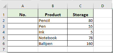
1. मूल डेटा की शुरुआत में एक नया कॉलम डालें। यहां मैं नीचे दिखाए गए स्क्रीनशॉट के अनुसार मूल डेटा से पहले कॉलम नंबर डालता हूं:

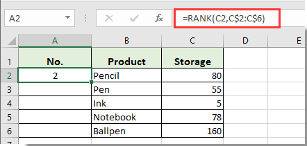
2. हमारे उदाहरण का अनुसरण करें, सूत्र दर्ज करें =रैंक(सी2,सी$2:सी$6) मूल उत्पादों को उनके भंडारण के आधार पर क्रमबद्ध करने के लिए सेल A2 में, और दबाएँ दर्ज कुंजी।

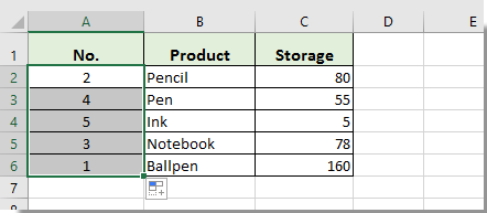
3. सेल A2 का चयन करते रहें, खींचें भरने वाला संचालक नंबर कॉलम में बाकी सभी नंबर पाने के लिए सेल A6 पर जाएं।

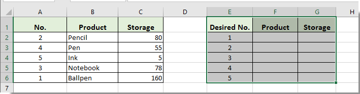
4: मूल डेटा के शीर्षकों की प्रतिलिपि बनाएँ, और फिर उन्हें मूल तालिका के अलावा चिपकाएँ, जैसे E1:G1। वांछित नंबर कॉलम में, नंबर ऑर्डर के समान अनुक्रम संख्याएं डालें जैसे 1, 2,…। स्क्रीनशॉट देखें:

5. सूत्र दर्ज करें =VLOOKUP(E2,A$2:C$6,2,FALSE) सेल F2 में, और दबाएँ दर्ज कुंजी।

यह सूत्र वांछित संख्या का मान खोजेगा। मूल तालिका में, और सेल में संबंधित उत्पाद का नाम प्रदर्शित करें।

नोट: यदि उत्पाद कॉलम या स्टोरेज कॉलम में दोहराव या संबंध प्रदर्शित होता है, तो बेहतर होगा कि आप इस फ़ंक्शन को लागू करें =IFERROR(VLOOKUP(E2,A$2:C$6,2,FALSE), VLOOKUP(E2,A$2:C$6,2,TRUE))

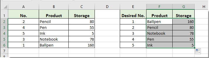
6. सेल F2 का चयन करते रहें, सभी उत्पाद नाम प्राप्त करने के लिए फिल हैंडल को सेल F6 तक नीचे खींचें, और रेंज F2:F6 का चयन करते रहें, सभी स्टोरेज नंबर प्राप्त करने के लिए फिल हैंडल को रेंज G2:G6 तक दाईं ओर खींचें।

फिर आपको नीचे स्क्रीनशॉट में दिखाए अनुसार स्टोरेज के अनुसार घटते क्रम में एक नई स्टोरेज टेबल मिलेगी:

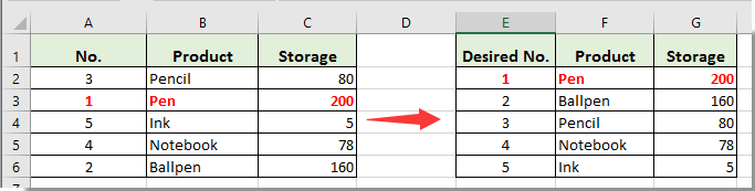
मान लीजिए कि आपकी स्टेशनरी की दुकान ने 145 और पेन खरीदे, और अब आपके पास कुल 200 पेन हैं। बस पेन के भंडारण की मूल तालिका को संशोधित करें, आप देखेंगे कि नई तालिका पलक झपकते ही अपडेट हो गई है, निम्न स्क्रीन शॉट देखें:

सर्वोत्तम कार्यालय उत्पादकता उपकरण

🤖 कुटूल्स एआई सहयोगी: निम्न के आधार पर डेटा विश्लेषण में क्रांति लाएं: बुद्धिमान निष्पादन   |  कोड जनरेट करें  |  कस्टम फ़ॉर्मूले बनाएं  |  डेटा का विश्लेषण करें और चार्ट बनाएं  |  कुटूल फ़ंक्शंस का आह्वान करें...
लोकप्रिय सुविधाएँ: डुप्लिकेट ढूंढें, हाइलाइट करें या पहचानें   |  रिक्त पंक्तियाँ हटाएँ   |  डेटा खोए बिना कॉलम या सेल को संयोजित करें   |   फॉर्मूला के बिना गोल ...
सुपर लुकअप: एकाधिक मानदंड VLookup    मल्टीपल वैल्यू वीलुकअप  |   अनेक शीटों में VLookup   |   फजी लुकअप ....
उन्नत ड्रॉप-डाउन सूची: शीघ्रता से ड्रॉप डाउन सूची बनाएं   |  आश्रित ड्रॉप डाउन सूची   |  बहु-चयन ड्रॉप डाउन सूची ....
स्तम्भ प्रबंधक: कॉलमों की एक विशिष्ट संख्या जोड़ें  |  कॉलम ले जाएँ  |  छिपे हुए कॉलम की दृश्यता स्थिति टॉगल करें  |  रेंज और कॉलम की तुलना करें ...
फीचर्ड फीचर्स: ग्रिड फोकस   |  डिजाइन देखें   |   बड़ा फॉर्मूला बार    कार्यपुस्तिका एवं शीट प्रबंधक   |  संसाधन लाइब्रेरी (ऑटो टेक्स्ट)   |  खजूर बीनने वाला   |  कार्यपत्रकों को संयोजित करें   |  एन्क्रिप्ट/डिक्रिप्ट सेल    सूची के अनुसार ईमेल भेजें   |  सुपर फ़िल्टर   |   विशेष फ़िल्टर (फ़िल्टर बोल्ड/इटैलिक/स्ट्राइकथ्रू...) ...
शीर्ष 15 टूलसेट12 टेक्स्ट टूल्स (पाठ जोड़ें, अक्षर हटाएँ, ...)   |   50 + चार्ट प्रकार (गैन्ट चार्ट, ...)   |   40+ प्रैक्टिकल सूत्र (जन्मदिन के आधार पर आयु की गणना करें, ...)   |   19 निवेशन टूल्स (QR कोड डालें, पथ से चित्र सम्मिलित करें, ...)   |   12 रूपांतरण टूल्स (शब्दों को संख्याएँ, मुद्रा रूपांतरण, ...)   |   7 विलय और विभाजन टूल्स (उन्नत संयोजन पंक्तियाँ, विभाजन कोशिकाओं, ...)   |   ... और अधिक

एक्सेल के लिए कुटूल के साथ अपने एक्सेल कौशल को सुपरचार्ज करें, और पहले जैसी दक्षता का अनुभव करें। एक्सेल के लिए कुटूल उत्पादकता बढ़ाने और समय बचाने के लिए 300 से अधिक उन्नत सुविधाएँ प्रदान करता है।  वह सुविधा प्राप्त करने के लिए यहां क्लिक करें जिसकी आपको सबसे अधिक आवश्यकता है...

Description


ऑफिस टैब ऑफिस में टैब्ड इंटरफ़ेस लाता है, और आपके काम को बहुत आसान बनाता है

  • Word, Excel, PowerPoint में टैब्ड संपादन और रीडिंग सक्षम करें, प्रकाशक, एक्सेस, विसियो और प्रोजेक्ट।
  • नई विंडो के बजाय एक ही विंडो के नए टैब में एकाधिक दस्तावेज़ खोलें और बनाएं।
  • आपकी उत्पादकता 50% बढ़ जाती है, और आपके लिए हर दिन सैकड़ों माउस क्लिक कम हो जाते हैं!
Comments (49)
No ratings yet. Be the first to rate!
This comment was minimized by the moderator on the site
hi,, what if there will be more than to numbers that were ties?
This comment was minimized by the moderator on the site
Wonderful....Thanks this helped me
This comment was minimized by the moderator on the site
I had lost the ability to sort several rows of information on one page of a spreadsheet with many pages. After trying to fix the situation by reworking formulas none of the information will sort now. Can I fix this without having to recreate page that is the problem. Same information needs to be transferred to another page that contains all information from all the pages; this too stops sort there. Big problem and don't know how to solve it.
This comment was minimized by the moderator on the site
i need to convert a number into another format.lets take an example - no =12394567 i need to convert it into 674501239. its simple (last 2 digit in first ,then 2nd last 2 digits then add a zero(0) then first four digits in the last. can you please guys tell me the formula for this?
This comment was minimized by the moderator on the site
=CONCATENATE(RIGHT(A1,2),MID(A1,5,2),"0",LEFT(A1,4)) will get you that order of digits.
This comment was minimized by the moderator on the site
you can use the CONCATENATE and then LEFT or RIGHT in excel formula. Its easy, Got it ?
This comment was minimized by the moderator on the site
Sure, mail me the detail and I will show you the finished product
This comment was minimized by the moderator on the site
Hi, no problem, email me and I will show hulu how the finished product works.
This comment was minimized by the moderator on the site
Hi Dear, I have a sheet with 100 items , each item has a specific cost that happens in one year .I want to create another sheet that shows only the item that has cost in one year automatically ? for example all of the item with item No. and description and cost in 2016 and then for 2017 and so on... thanks
This comment was minimized by the moderator on the site
how can i sort lowest to highest value (a to z) in your example i.e lowest storage to highest storage. i use your formulla '=RANK(C2,C$2:C $6) + COUNTIF(C$2:C2, "="&C2)-1'" & "=IFERROR(VLOOKUP(E2,A$2:C$6,2,FALSE), VLOOKUP(E2,A$2:C$6,2,TRUE))" . al is going well but i cannot sort lowest to highest.
This comment was minimized by the moderator on the site
Kedirech, you rock!! The COUNT thing eliminates ties!! I've had this problem for years but now this is the solution!! Thanks!!
This comment was minimized by the moderator on the site
Hi, I do it with if statements alone, how do I let you look at my file?
There are no comments posted here yet
Load More
Please leave your comments in English
Posting as Guest
×
Rate this post:
0   Characters
Suggested Locations