मुख्य सामग्री पर जाएं

Google शीट में किसी कॉलम में घटनाओं की संख्या कैसे गिनें?

लेखक: ज़ियाओयांग अंतिम संशोधित: 2020-04-23

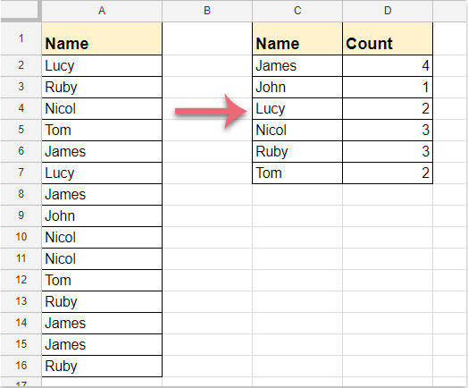
मान लीजिए, आपके पास Google शीट के कॉलम ए में नामों की एक सूची है, और अब, आप यह गिनना चाहते हैं कि प्रत्येक अद्वितीय नाम कितनी बार नीचे दिखाए गए स्क्रीनशॉट के अनुसार दिखाई देता है। इस ट्यूटोरियल में, मैं Google शीट में इस कार्य को हल करने के लिए कुछ सूत्रों के बारे में बात करूंगा।

सहायक सूत्र के साथ Google शीट में एक कॉलम में घटनाओं की संख्या की गणना करें

सूत्र के साथ Google शीट में एक कॉलम में घटनाओं की संख्या की गणना करें


सहायक सूत्र के साथ Google शीट में एक कॉलम में घटनाओं की संख्या की गणना करें

इस विधि में, आप पहले कॉलम से सभी अद्वितीय नाम निकाल सकते हैं, और फिर अद्वितीय मान के आधार पर घटना की गणना कर सकते हैं।

1. कृपया यह सूत्र दर्ज करें: = सिंगल (ए 2: ए 16) एक रिक्त कक्ष में जहाँ आप अद्वितीय नाम निकालना चाहते हैं, और फिर दबाएँ दर्ज कुंजी, सभी अद्वितीय मान दिखाए गए स्क्रीनशॉट के अनुसार सूचीबद्ध किए गए हैं:

नोट: उपरोक्त सूत्र में, A2: A16 वह कॉलम डेटा है जिसे आप गिनना चाहते हैं।

2. और फिर इस सूत्र में प्रवेश करते जाएँ: =COUNTIF(A2:A16, C2) प्रथम सूत्र कक्ष के पास, दबाएँ दर्ज पहला परिणाम प्राप्त करने के लिए कुंजी, और फिर भरण हैंडल को उन कक्षों तक नीचे खींचें जिन्हें आप अद्वितीय मानों की घटना की गणना करना चाहते हैं, स्क्रीनशॉट देखें:

नोट: उपरोक्त सूत्र में, A2: A16 वह कॉलम डेटा है जिससे आप अद्वितीय नाम गिनना चाहते हैं, और C2 यह आपके द्वारा निकाला गया पहला अद्वितीय मान है।


सूत्र के साथ Google शीट में एक कॉलम में घटनाओं की संख्या की गणना करें

परिणाम प्राप्त करने के लिए आप निम्न सूत्र भी लागू कर सकते हैं। कृपया इस प्रकार करें:

कृपया यह सूत्र दर्ज करें: =ArrayFormula(QUERY(A1:A16&{"",""},"Col1 चुनें, गिनती(Col2) जहां Col1 != '' समूह by Col1 लेबल गिनती(Col2) 'गिनती'",1)) एक रिक्त कक्ष में जहाँ आप परिणाम डालना चाहते हैं, फिर दबाएँ दर्ज कुंजी, और परिकलित परिणाम तुरंत प्रदर्शित हो गया है, स्क्रीनशॉट देखें:

नोट: उपरोक्त सूत्र में, A1: A16 वह डेटा श्रेणी है जिसमें वह कॉलम हेडर भी शामिल है जिसे आप गिनना चाहते हैं।


Microsoft Excel में किसी कॉलम में घटनाओं की संख्या की गणना करें:

एक्सेल के लिए कुटूलहै उन्नत संयोजन पंक्तियाँ उपयोगिता आपको किसी कॉलम में घटनाओं की संख्या गिनने में मदद कर सकती है, और यह आपको किसी अन्य कॉलम में समान सेल के आधार पर संबंधित सेल मानों को संयोजित या योग करने में भी मदद कर सकती है।

एक्सेल के लिए कुटूल: 300 से अधिक उपयोगी एक्सेल ऐड-इन्स के साथ, 30 दिनों में बिना किसी सीमा के आज़माने के लिए निःशुल्क। अभी डाउनलोड करें और निःशुल्क परीक्षण करें!

सर्वोत्तम कार्यालय उत्पादकता उपकरण

🤖 कुटूल्स एआई सहयोगी: निम्न के आधार पर डेटा विश्लेषण में क्रांति लाएं: बुद्धिमान निष्पादन   |  कोड जनरेट करें  |  कस्टम फ़ॉर्मूले बनाएं  |  डेटा का विश्लेषण करें और चार्ट बनाएं  |  कुटूल फ़ंक्शंस का आह्वान करें...
लोकप्रिय सुविधाएँ: डुप्लिकेट ढूंढें, हाइलाइट करें या पहचानें   |  रिक्त पंक्तियाँ हटाएँ   |  डेटा खोए बिना कॉलम या सेल को संयोजित करें   |   फॉर्मूला के बिना गोल ...
सुपर लुकअप: एकाधिक मानदंड VLookup    मल्टीपल वैल्यू वीलुकअप  |   अनेक शीटों में VLookup   |   फजी लुकअप ....
उन्नत ड्रॉप-डाउन सूची: शीघ्रता से ड्रॉप डाउन सूची बनाएं   |  आश्रित ड्रॉप डाउन सूची   |  बहु-चयन ड्रॉप डाउन सूची ....
स्तम्भ प्रबंधक: कॉलमों की एक विशिष्ट संख्या जोड़ें  |  कॉलम ले जाएँ  |  छिपे हुए कॉलम की दृश्यता स्थिति टॉगल करें  |  रेंज और कॉलम की तुलना करें ...
फीचर्ड फीचर्स: ग्रिड फोकस   |  डिजाइन देखें   |   बड़ा फॉर्मूला बार    कार्यपुस्तिका एवं शीट प्रबंधक   |  संसाधन लाइब्रेरी (ऑटो टेक्स्ट)   |  खजूर बीनने वाला   |  कार्यपत्रकों को संयोजित करें   |  एन्क्रिप्ट/डिक्रिप्ट सेल    सूची के अनुसार ईमेल भेजें   |  सुपर फ़िल्टर   |   विशेष फ़िल्टर (फ़िल्टर बोल्ड/इटैलिक/स्ट्राइकथ्रू...) ...
शीर्ष 15 टूलसेट12 टेक्स्ट टूल्स (पाठ जोड़ें, अक्षर हटाएँ, ...)   |   50 + चार्ट प्रकार (गैन्ट चार्ट, ...)   |   40+ प्रैक्टिकल सूत्र (जन्मदिन के आधार पर आयु की गणना करें, ...)   |   19 निवेशन टूल्स (QR कोड डालें, पथ से चित्र सम्मिलित करें, ...)   |   12 रूपांतरण टूल्स (शब्दों को संख्याएँ, मुद्रा रूपांतरण, ...)   |   7 विलय और विभाजन टूल्स (उन्नत संयोजन पंक्तियाँ, विभाजन कोशिकाओं, ...)   |   ... और अधिक

एक्सेल के लिए कुटूल के साथ अपने एक्सेल कौशल को सुपरचार्ज करें, और पहले जैसी दक्षता का अनुभव करें। एक्सेल के लिए कुटूल उत्पादकता बढ़ाने और समय बचाने के लिए 300 से अधिक उन्नत सुविधाएँ प्रदान करता है।  वह सुविधा प्राप्त करने के लिए यहां क्लिक करें जिसकी आपको सबसे अधिक आवश्यकता है...

Description


ऑफिस टैब ऑफिस में टैब्ड इंटरफ़ेस लाता है, और आपके काम को बहुत आसान बनाता है

  • Word, Excel, PowerPoint में टैब्ड संपादन और रीडिंग सक्षम करें, प्रकाशक, एक्सेस, विसियो और प्रोजेक्ट।
  • नई विंडो के बजाय एक ही विंडो के नए टैब में एकाधिक दस्तावेज़ खोलें और बनाएं।
  • आपकी उत्पादकता 50% बढ़ जाती है, और आपके लिए हर दिन सैकड़ों माउस क्लिक कम हो जाते हैं!
Comments (14)
No ratings yet. Be the first to rate!
This comment was minimized by the moderator on the site
可以限制规定内容出现的频次吗
This comment was minimized by the moderator on the site
Thanks!!! how do I count multiple columns?Ie column A, B,C,D all have names that needs to be counted
This comment was minimized by the moderator on the site
Thank you for this! Been trying to figure it out for hours!
This comment was minimized by the moderator on the site
Hi, I am trying to filter out some data from a sheet that is regularly updated. To simplify keeping track of the data I have a reporting section on the google sheet.The problem is that the data isn't organized in the most ideal way.

There are 2 columns that I want to use specific data from to create a filter, then with the leftover names I want to know how many unique names there are


Column 1 - Filter with A for one report field, B for the other report field (I will manually change this in the formula)

Column 2 - There are 9 Text entries possible. I want to only include 3 of them as a Filter

Column 3 - There are a couple of thousand entries(names), many are the same in multiple rows. With the data filtered using Column 1, and Column 2, I want to get a number for how many unique names are left after the data has been filtered.


I am not used to having this many things I am trying to filter the data from so any help would be hugely appreciated.


Have an excellent day
This comment was minimized by the moderator on the site
I have a google sheet with a lot of information but I am looking to filter it down into a report.

Column1 - Options are A, B (The is the first data to sort)
Column 2 - has 3 of the text string that I want my sum to include, but I want to leave out the others 5.
Column 3 - Names that I want to know how many unique names there are

What I am looking to figure out is the following

Option A, the sum to only include 3 text string that appears multiple times in a 2nd column, The total being how many unique names there are in Column 3

Hoping someone can help as this is a bit over my experience level
This comment was minimized by the moderator on the site
My count isn't grouping the names together.
i.e.
Column B says
Independence
Walnut St.
Parkway
Walnut St.
and instead of my " count " column saying Walnut St. 2 it says
Walnut St. 1
Walnut St. 1

How can I fix this ?
This comment was minimized by the moderator on the site
This is partly what I'm looking for.
Now my next issue is, how can I sort these so that I get them in desending order?
So it should be looking like this:
James 4
Nicol 3
Ruby 3
Lucy 2
Tom 2
John 1

Hope you can help with that as well
This comment was minimized by the moderator on the site
Hi,
If you want to sort the results in descending order, you just need to sort the data by the formula result column after getting the result.
Hope it can help you!
This comment was minimized by the moderator on the site
Whenever I try to sort, I get an error, is there a way I can fix that? I have the $A$1:$A$7, B1 as my formula - is there something in my formula I should edit?
This comment was minimized by the moderator on the site
VERY useful - thank you so much!
This comment was minimized by the moderator on the site
Thanks! Super useful!
This comment was minimized by the moderator on the site
When you drag the handle down to apply it to the rest of the values, it increments the search radius by 1. So if youre searching =COUNTIF(A1:A10,C1), when you drag the handle down, the second value will be =COUNTIF(A2:A11,C2).
This comment was minimized by the moderator on the site
This is SOOO helpful! This skips an entire step
This comment was minimized by the moderator on the site
You fix it this way
=COUNTIF($A$2:$A$11,C2)
There are no comments posted here yet
Please leave your comments in English
Posting as Guest
×
Rate this post:
0   Characters
Suggested Locations