मुख्य सामग्री पर जाएं

Google शीट में आश्रित ड्रॉप डाउन सूची कैसे बनाएं?

लेखक: ज़ियाओयांग अंतिम संशोधित: 2020-11-25

Google शीट में सामान्य ड्रॉप डाउन सूची डालना आपके लिए एक आसान काम हो सकता है, लेकिन, कभी-कभी, आपको एक आश्रित ड्रॉप डाउन सूची डालने की आवश्यकता हो सकती है जिसका अर्थ है पहली ड्रॉप डाउन सूची की पसंद के आधार पर दूसरी ड्रॉप डाउन सूची। आप Google शीट में इस कार्य से कैसे निपट सकते हैं?

Google शीट में एक आश्रित ड्रॉप डाउन सूची बनाएं


Google शीट में एक आश्रित ड्रॉप डाउन सूची बनाएं

निम्नलिखित चरण आपको आश्रित ड्रॉप डाउन सूची सम्मिलित करने में मदद कर सकते हैं, कृपया ऐसा करें:

1. सबसे पहले, आपको मूल ड्रॉप डाउन सूची डालनी चाहिए, कृपया उस सेल का चयन करें जहां आप पहली ड्रॉप डाउन सूची डालना चाहते हैं, और फिर क्लिक करें जानकारी > डेटा मान्य, स्क्रीनशॉट देखें:

2. बाहर निकले में डेटा मान्य संवाद बॉक्स में, चयन करें एक श्रेणी से सूची के बगल में ड्रॉप डाउन सूची से मापदंड अनुभाग, और फिर क्लिक करें उन सेल मानों का चयन करने के लिए बटन, जिनके आधार पर आप पहली ड्रॉप डाउन सूची बनाना चाहते हैं, स्क्रीनशॉट देखें:

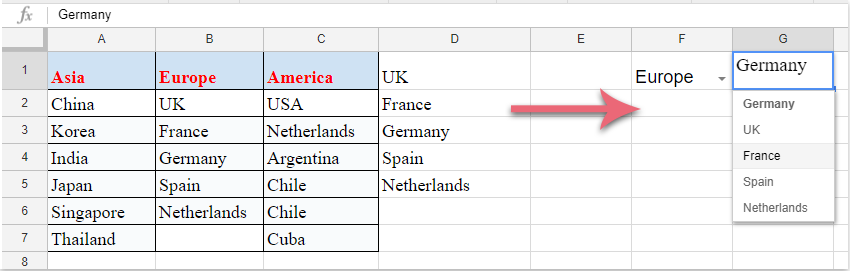
3। तब दबायें सहेजें बटन, पहली ड्रॉप डाउन सूची बनाई गई है। बनाई गई ड्रॉप डाउन सूची से एक आइटम चुनें, और फिर यह सूत्र दर्ज करें: =arrayformula(if(F1=A1,A2:A7,if(F1=B1,B2:B6,if(F1=C1,C2:C7,"")))) एक रिक्त सेल में जो डेटा कॉलम से सटा हुआ है, फिर दबाएँ दर्ज कुंजी, पहली ड्रॉप डाउन सूची आइटम के आधार पर सभी मिलान मान एक ही बार में प्रदर्शित किए गए हैं, स्क्रीनशॉट देखें:

नोट: उपरोक्त सूत्र में: F1 पहला ड्रॉप डाउन सूची सेल है, A1, B1 और C1 पहली ड्रॉप डाउन सूची के आइटम हैं, A2: A7, B2: B6 और सी2:सी7 वे सेल मान हैं जिन पर दूसरी ड्रॉप डाउन सूची आधारित है। आप उन्हें अपने हिसाब से बदल सकते हैं.

4. और फिर आप दूसरी आश्रित ड्रॉप डाउन सूची बना सकते हैं, उस सेल पर क्लिक करें जहां आप दूसरी ड्रॉप डाउन सूची रखना चाहते हैं, और फिर क्लिक करें जानकारी > डेटा मान्य पर जाने के लिए डेटा मान्य संवाद बॉक्स, चुनें एक श्रेणी से सूची बगल में ड्रॉप डाउन से मापदंड अनुभाग, और सूत्र कक्षों का चयन करने के लिए बटन पर क्लिक करें जो पहले ड्रॉप डाउन आइटम के मिलान परिणाम हैं, स्क्रीनशॉट देखें:

5. अंत में, सेव बटन पर क्लिक करें, और दूसरी आश्रित ड्रॉप डाउन सूची सफलतापूर्वक बनाई गई है जैसा कि निम्नलिखित स्क्रीनशॉट में दिखाया गया है:

सर्वोत्तम कार्यालय उत्पादकता उपकरण

🤖 कुटूल्स एआई सहयोगी: निम्न के आधार पर डेटा विश्लेषण में क्रांति लाएं: बुद्धिमान निष्पादन   |  कोड जनरेट करें  |  कस्टम फ़ॉर्मूले बनाएं  |  डेटा का विश्लेषण करें और चार्ट बनाएं  |  कुटूल फ़ंक्शंस का आह्वान करें...
लोकप्रिय सुविधाएँ: डुप्लिकेट ढूंढें, हाइलाइट करें या पहचानें   |  रिक्त पंक्तियाँ हटाएँ   |  डेटा खोए बिना कॉलम या सेल को संयोजित करें   |   फॉर्मूला के बिना गोल ...
सुपर लुकअप: एकाधिक मानदंड VLookup    मल्टीपल वैल्यू वीलुकअप  |   अनेक शीटों में VLookup   |   फजी लुकअप ....
उन्नत ड्रॉप-डाउन सूची: शीघ्रता से ड्रॉप डाउन सूची बनाएं   |  आश्रित ड्रॉप डाउन सूची   |  बहु-चयन ड्रॉप डाउन सूची ....
स्तम्भ प्रबंधक: कॉलमों की एक विशिष्ट संख्या जोड़ें  |  कॉलम ले जाएँ  |  छिपे हुए कॉलम की दृश्यता स्थिति टॉगल करें  |  रेंज और कॉलम की तुलना करें ...
फीचर्ड फीचर्स: ग्रिड फोकस   |  डिजाइन देखें   |   बड़ा फॉर्मूला बार    कार्यपुस्तिका एवं शीट प्रबंधक   |  संसाधन लाइब्रेरी (ऑटो टेक्स्ट)   |  खजूर बीनने वाला   |  कार्यपत्रकों को संयोजित करें   |  एन्क्रिप्ट/डिक्रिप्ट सेल    सूची के अनुसार ईमेल भेजें   |  सुपर फ़िल्टर   |   विशेष फ़िल्टर (फ़िल्टर बोल्ड/इटैलिक/स्ट्राइकथ्रू...) ...
शीर्ष 15 टूलसेट12 टेक्स्ट टूल्स (पाठ जोड़ें, अक्षर हटाएँ, ...)   |   50 + चार्ट प्रकार (गैन्ट चार्ट, ...)   |   40+ प्रैक्टिकल सूत्र (जन्मदिन के आधार पर आयु की गणना करें, ...)   |   19 निवेशन टूल्स (QR कोड डालें, पथ से चित्र सम्मिलित करें, ...)   |   12 रूपांतरण टूल्स (शब्दों को संख्याएँ, मुद्रा रूपांतरण, ...)   |   7 विलय और विभाजन टूल्स (उन्नत संयोजन पंक्तियाँ, विभाजन कोशिकाओं, ...)   |   ... और अधिक

एक्सेल के लिए कुटूल के साथ अपने एक्सेल कौशल को सुपरचार्ज करें, और पहले जैसी दक्षता का अनुभव करें। एक्सेल के लिए कुटूल उत्पादकता बढ़ाने और समय बचाने के लिए 300 से अधिक उन्नत सुविधाएँ प्रदान करता है।  वह सुविधा प्राप्त करने के लिए यहां क्लिक करें जिसकी आपको सबसे अधिक आवश्यकता है...

Description


ऑफिस टैब ऑफिस में टैब्ड इंटरफ़ेस लाता है, और आपके काम को बहुत आसान बनाता है

  • Word, Excel, PowerPoint में टैब्ड संपादन और रीडिंग सक्षम करें, प्रकाशक, एक्सेस, विसियो और प्रोजेक्ट।
  • नई विंडो के बजाय एक ही विंडो के नए टैब में एकाधिक दस्तावेज़ खोलें और बनाएं।
  • आपकी उत्पादकता 50% बढ़ जाती है, और आपके लिए हर दिन सैकड़ों माउस क्लिक कम हो जाते हैं!
Comments (18)
No ratings yet. Be the first to rate!
This comment was minimized by the moderator on the site
Hi there. Its been working but for it only appears that only one cell can be formulated.I need help 
For example: in Cell A1, it shows dependent dropdown, but when in cell a2 it does not work.
Thas what help that i need, From A:A, They have all different selection from the dropdown list. Thanks.
This comment was minimized by the moderator on the site
Would it been possible to create pull down menu based of formula?
I use formula "=SUMIFS(Items!$I:$I,Items!$A:$A,K$1,Items!$D:$D,$D2)" (=for example 150) to find the qty on pallet based on item and container size.
So I wanted to create pull down menu like qty 1 pallet, qty 2 pallets, qty 3 pallets,.....
Then user will always order qty of full pallets like 150, 2 x 150, 3 x150, up to 21 x 150.
This comment was minimized by the moderator on the site
Hi, I already created a drop down list like this one, what I'd like to know is how i can, when clicking on one option from that list, restrict what appears as options on another cell. For example, in one cell i can choose between laparoscopy and orthopaedics. If I choose orthopaedics then, the other cell which has a list of doctors, should only show the doctors for orthopedy and not all of them. Does anyone know how to do this?
This comment was minimized by the moderator on the site
Hii Sir,
I Want to Create A Dependent Drop Down List Like
- State(A1):- District(B1):- Taluka(C1) :- Then Information(D1) ,
So I need your Help .
Tell How do you do this Type of Dependent Drop down List in Excel or Google Sheet
This comment was minimized by the moderator on the site
Hi, Shelate,
Maybe the below article can solve your problem, please view it:
https://www.extendoffice.com/documents/excel/5852-excel-multiple-level-drop-down-list.html

Please try, hope it can help you!
This comment was minimized by the moderator on the site
Now is needed to use: =arrayformula(if(F1=A1;A2:A7;if(F1=B1;B2:B6;if(F1=C1;C2:C7;""))))
This comment was minimized by the moderator on the site
Thank you soooo much!
This comment was minimized by the moderator on the site
Hi,
I was wondering if anyone could advise me with this? I've followed the above steps but on step 3 rather than getting:
"...all the matching values based on the first drop down list item have been displayed at once," I am just seeing one value (the top one from the drop down list).
My cells are placed slightly differently and the first drop down is filled from another sheet (from anywhere int eh column excluding the top row) so my formula is:

=arrayformula(if(VLE!D2:D=B11,B12,if(VLE!D2:D=C11,C12:C14,if(VLE!D2:D=D11,D12:D14,if(VLE!D2:D=E11,E12:E16,if(VLE!D2:D=F11,F12:F16,""))))))

It is correctly displaying the top drop down option for each of (using cell numbers from the step 3 example on this page) A1, B1, and C1 so, again using this page's example, if I select Asia form the F1 drop down, I would get China, but nothing further


Any suggestions?

Many thanks! Nick
This comment was minimized by the moderator on the site
If the first drop own is on sheet 1 A1, will this work were I want the second drop down as sheet 1 A2, but to have its data range on a separate sheet?
This comment was minimized by the moderator on the site
Ich bekomm immer die Meldung "Fehler beim Parsen der Formel" wenn ich =arrayformula(if(F1=A1,A2:A7,if(F1=B1,B2:B6,if(F1=C1,C2:C7,"")))) eingebe. Was ist der "Weiter-Schlüsel"? Reicht es nicht wie bei Excel die Formel einzugeben?
This comment was minimized by the moderator on the site
Ersetzen Sie den , zu ;
es hat für mich funktioniert
This comment was minimized by the moderator on the site
This is the best explanation I have found, so thank you for that!

In my situation, I am working with over 200 rows with more being continuously added. Is there an easier/more efficient way to handle this many rows?
This comment was minimized by the moderator on the site
Yes, if you don't put number index to specify ending cell.
Like instead of C2:C7 you put C2:C. This will automatically tell the array formula, that you want to consider all values in column "C" starting at "C2".
This comment was minimized by the moderator on the site
What happens if I want exactly the same dropdown list in F2 as you have in F1 ?
I tried, and it doesn't overwrite D1:D7 .. meaning D1:D7 is only available once.
I need something else, double dropdown, but on many-many lines .. guess I must use another system then .. not sure which ..
This comment was minimized by the moderator on the site
Hi, Xained,
This method can only applied to one cell, if you have some good ways for applying this to multiple cells, please comment here.

Thank you!
This comment was minimized by the moderator on the site
Please, guide me how to do that.Thanks
This comment was minimized by the moderator on the site
혹시, 하나의 셀이 아닌 여러셀에 할 수 있는 방법을 알 수 있을까요?
This comment was minimized by the moderator on the site
내말이... 시바 좃빠지게 따라했디만 밑에줄은 안되노..
There are no comments posted here yet
Please leave your comments in English
Posting as Guest
×
Rate this post:
0   Characters
Suggested Locations