मुख्य सामग्री पर जाएं

Excel में पंक्तियाँ सम्मिलित करते समय सूत्र को कैसे अद्यतन करें? 

लेखक: ज़ियाओयांग अंतिम संशोधित: 2020-12-11
दस्तावेज़ अद्यतन सूत्र पंक्तियाँ 1 सम्मिलित करना

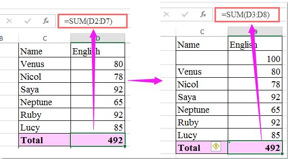
उदाहरण के लिए, मेरे पास सेल D2 में एक सूत्र =sum(D7:D8) है, अब, जब मैं दूसरी पंक्ति में एक पंक्ति डालता हूं और नया नंबर दर्ज करता हूं, तो सूत्र स्वचालित रूप से =sum(D3:D8) में बदल जाएगा जिसमें शामिल नहीं है सेल D2 निम्न स्क्रीनशॉट के अनुसार दिखाया गया है। इस मामले में, जब भी मैं पंक्तियाँ सम्मिलित करता हूँ तो मुझे हर बार सूत्र में सेल संदर्भ को बदलना पड़ता है। Excel में पंक्तियाँ सम्मिलित करते समय मैं हमेशा सेल D2 से शुरू होने वाली संख्याओं का योग कैसे कर सकता हूँ?

सूत्र के साथ पंक्तियों को स्वचालित रूप से सम्मिलित करते समय सूत्र को अद्यतन करें


तीर नीला दायां बुलबुला सूत्र के साथ पंक्तियों को स्वचालित रूप से सम्मिलित करते समय सूत्र को अद्यतन करें

निम्नलिखित सरल सूत्र आपको नई पंक्तियाँ सम्मिलित करते समय सेल संदर्भ को मैन्युअल रूप से बदले बिना सूत्र को स्वचालित रूप से अपडेट करने में मदद कर सकता है, कृपया ऐसा करें:

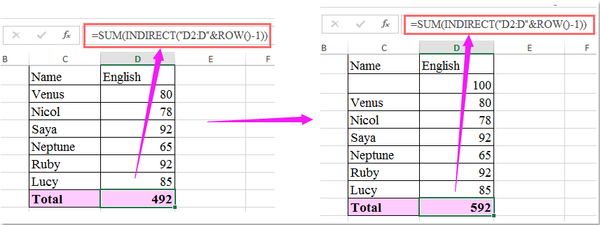
1. यह सूत्र दर्ज करें: =SUM(अप्रत्यक्ष("D2:D"&ROW()-1)) (D2 यह सूची में पहला कक्ष है जिसका आप योग करना चाहते हैं) उन कक्षों के अंत में जिनका आप संख्या सूची में योग करना चाहते हैं, और दबाएँ दर्ज कुंजी।

2. और अब, जब आप संख्या सूची के बीच कहीं भी पंक्तियाँ सम्मिलित करेंगे, तो सूत्र स्वचालित रूप से अपडेट हो जाएगा, स्क्रीनशॉट देखें:

दस्तावेज़ अद्यतन सूत्र पंक्तियाँ 2 सम्मिलित करना

टिप्स: सूत्र तभी सही ढंग से काम करता है जब आप इसे डेटा सूची के अंत में रखते हैं।

सर्वोत्तम कार्यालय उत्पादकता उपकरण

🤖 कुटूल्स एआई सहयोगी: निम्न के आधार पर डेटा विश्लेषण में क्रांति लाएं: बुद्धिमान निष्पादन   |  कोड जनरेट करें  |  कस्टम फ़ॉर्मूले बनाएं  |  डेटा का विश्लेषण करें और चार्ट बनाएं  |  कुटूल फ़ंक्शंस का आह्वान करें...
लोकप्रिय सुविधाएँ: डुप्लिकेट ढूंढें, हाइलाइट करें या पहचानें   |  रिक्त पंक्तियाँ हटाएँ   |  डेटा खोए बिना कॉलम या सेल को संयोजित करें   |   फॉर्मूला के बिना गोल ...
सुपर लुकअप: एकाधिक मानदंड VLookup    मल्टीपल वैल्यू वीलुकअप  |   अनेक शीटों में VLookup   |   फजी लुकअप ....
उन्नत ड्रॉप-डाउन सूची: शीघ्रता से ड्रॉप डाउन सूची बनाएं   |  आश्रित ड्रॉप डाउन सूची   |  बहु-चयन ड्रॉप डाउन सूची ....
स्तम्भ प्रबंधक: कॉलमों की एक विशिष्ट संख्या जोड़ें  |  कॉलम ले जाएँ  |  छिपे हुए कॉलम की दृश्यता स्थिति टॉगल करें  |  रेंज और कॉलम की तुलना करें ...
फीचर्ड फीचर्स: ग्रिड फोकस   |  डिजाइन देखें   |   बड़ा फॉर्मूला बार    कार्यपुस्तिका एवं शीट प्रबंधक   |  संसाधन लाइब्रेरी (ऑटो टेक्स्ट)   |  खजूर बीनने वाला   |  कार्यपत्रकों को संयोजित करें   |  एन्क्रिप्ट/डिक्रिप्ट सेल    सूची के अनुसार ईमेल भेजें   |  सुपर फ़िल्टर   |   विशेष फ़िल्टर (फ़िल्टर बोल्ड/इटैलिक/स्ट्राइकथ्रू...) ...
शीर्ष 15 टूलसेट12 टेक्स्ट टूल्स (पाठ जोड़ें, अक्षर हटाएँ, ...)   |   50 + चार्ट प्रकार (गैन्ट चार्ट, ...)   |   40+ प्रैक्टिकल सूत्र (जन्मदिन के आधार पर आयु की गणना करें, ...)   |   19 निवेशन टूल्स (QR कोड डालें, पथ से चित्र सम्मिलित करें, ...)   |   12 रूपांतरण टूल्स (शब्दों को संख्याएँ, मुद्रा रूपांतरण, ...)   |   7 विलय और विभाजन टूल्स (उन्नत संयोजन पंक्तियाँ, विभाजन कोशिकाओं, ...)   |   ... और अधिक

एक्सेल के लिए कुटूल के साथ अपने एक्सेल कौशल को सुपरचार्ज करें, और पहले जैसी दक्षता का अनुभव करें। एक्सेल के लिए कुटूल उत्पादकता बढ़ाने और समय बचाने के लिए 300 से अधिक उन्नत सुविधाएँ प्रदान करता है।  वह सुविधा प्राप्त करने के लिए यहां क्लिक करें जिसकी आपको सबसे अधिक आवश्यकता है...

Description


ऑफिस टैब ऑफिस में टैब्ड इंटरफ़ेस लाता है, और आपके काम को बहुत आसान बनाता है

  • Word, Excel, PowerPoint में टैब्ड संपादन और रीडिंग सक्षम करें, प्रकाशक, एक्सेस, विसियो और प्रोजेक्ट।
  • नई विंडो के बजाय एक ही विंडो के नए टैब में एकाधिक दस्तावेज़ खोलें और बनाएं।
  • आपकी उत्पादकता 50% बढ़ जाती है, और आपके लिए हर दिन सैकड़ों माउस क्लिक कम हो जाते हैं!
Comments (9)
No ratings yet. Be the first to rate!
This comment was minimized by the moderator on the site
Thank you very much.
This comment was minimized by the moderator on the site
Hello,
You are welcome. Glad it helps. Any questions, please feel free to contact us. Have a great day.
Sincerely,
Mandy
This comment was minimized by the moderator on the site
Please help me with Excel formula that update automatically without changing the cell reference manually when inserting new row at the bottom only. But not when inserting new row at the top. Thanks
This comment was minimized by the moderator on the site
This is really helpful ... except it does not update the row/column when copying and pasting this formula, so if I have a bunch of them, I have to update the column/row manually (like in the example, if I copy this to the adjacent column E, it still has D ...)

Unless someone knows a workaround to that problem, too?
This comment was minimized by the moderator on the site
you can use a different formula SUM(D$2:D12) as you insert a new row it continues to sum it up
This comment was minimized by the moderator on the site
I found that this only works if there is more than 1 row to total at the start.  Any ideas how you would do this for totalling 1 row to start and then adding in rows as you work on the spreadsheet?

This comment was minimized by the moderator on the site
You are the best! It works!
This comment was minimized by the moderator on the site
I have a simple cell reference in one of my cells down a column e.g.:"=H6", “=H7” etc. When I insert a row in Excel and copy formulas from row above, the cell reference in 'Opening Stock' does not update automatically in the row after the new blank row (should be equal to previous row balance, which is 60 now). But it updates correctly in all other rows below. Is there a way to force Excel to update cell reference to the cell in blank row above? Have searched the web, but did not get any satisfactory answer. I do not want to convert the data to a table, since it messes up the filters and formatting. Macros don't solve the problem either - they don't copy to the row following the blank one. Can anyone please help?
This comment was minimized by the moderator on the site
Hi Rayan!

Please if you see this let me know! You are the only one I found online who brought this issue up. However, my data is table not normal range. The automatic filling of the formula really helps and copy/pasting is a hassle. Anyway, when insert a row, the formulas update for all columns except one! In the row and the cell, instead of the formula shifting from =if(C24 = C25) to =if(C25 = C26), it goes to =if(C24 = C26) although C24 is not fixed!!! I've really tried all possible solutions...................
There are no comments posted here yet
Please leave your comments in English
Posting as Guest
×
Rate this post:
0   Characters
Suggested Locations