मुख्य सामग्री पर जाएं

एक्सेल में केवल सेल वैल्यू का हिस्सा कैसे छिपाएं?

लेखक: रवि अंतिम संशोधित: 2020-05-27
दस्तावेज़ आंशिक रूप से छिपाएँ 1
मान लीजिए कि आपके पास कर्मचारियों के बारे में कुछ सामान्य जानकारी वाली एक शीट है, लेकिन कुछ निजी हैं जैसे कि सामाजिक सुरक्षा नंबर। अब आप इन सामाजिक सुरक्षा नंबरों का हिस्सा छिपाना चाहते हैं जैसा कि नीचे स्क्रीनशॉट में दिखाया गया है, आप इसे जल्दी कैसे हल कर सकते हैं?

फ़ॉर्मेट सेल के साथ सामाजिक सुरक्षा नंबरों को आंशिक रूप से छिपाएं

सूत्रों के साथ पाठ या संख्या को आंशिक रूप से छिपाएँ

तीर नीला दायां बुलबुला फ़ॉर्मेट सेल के साथ सामाजिक सुरक्षा नंबरों को आंशिक रूप से छिपाएं

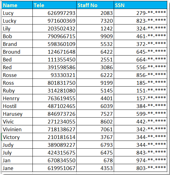
एक्सेल में सामाजिक सुरक्षा नंबरों के भाग को छिपाने के लिए, आप इसे हल करने के लिए फ़ॉर्मेट सेल लागू कर सकते हैं।

1. उन नंबरों का चयन करें जिन्हें आप आंशिक रूप से छिपाना चाहते हैं, और चयन करने के लिए राइट क्लिक करें प्रारूप प्रकोष्ठों संदर्भ मेनू से. स्क्रीनशॉट देखें:
दस्तावेज़ आंशिक रूप से छिपाएँ 2

2. फिर में प्रारूप प्रकोष्ठों संवाद, क्लिक करें नंबर टैब, और चयन रिवाज से वर्ग फलक, और इसे दर्ज करने के लिए जाएं 000,,"-**-****" में प्रकार दाहिने भाग में बॉक्स. स्क्रीनशॉट देखें:
दस्तावेज़ आंशिक रूप से छिपाएँ 3

3। क्लिक करें OK, अब आपके द्वारा चयनित आंशिक संख्याएँ छिपा दी गई हैं।

नोट:यदि चौथी संख्या 5 से बड़ी या उसके बराबर है तो यह संख्या को पूर्णांकित कर देगा।


तीर नीला दायां बुलबुला सूत्रों के साथ पाठ या संख्या को आंशिक रूप से छिपाएँ

उपरोक्त विधि से, आप केवल आंशिक संख्याएँ छिपा सकते हैं, यदि आप आंशिक संख्याएँ या पाठ छिपाना चाहते हैं, तो आप नीचे दिए अनुसार कर सकते हैं:

यहां हम पासपोर्ट नंबर के पहले 4 नंबर छुपाते हैं।

पासपोर्ट नंबर के आगे एक खाली सेल चुनें, उदाहरण के लिए F22, यह फॉर्मूला दर्ज करें = "****" और दाएँ(E22,5), और फिर इस फॉर्मूले को लागू करने के लिए आपको जिस सेल की आवश्यकता है उस पर ऑटोफिल हैंडल को खींचें।
दस्तावेज़ आंशिक रूप से छिपाएँ 4

सुझाव:

यदि आप अंतिम चार संख्याओं को छिपाना चाहते हैं, तो इस सूत्र का उपयोग करें, = बाएँ(H2,5)&"****"

यदि आप बीच की तीन संख्याओं को छिपाना चाहते हैं, तो इसका उपयोग करें =बाएं(H2,3)&"***"&दाएं(H2,3)

सर्वोत्तम कार्यालय उत्पादकता उपकरण

🤖 कुटूल्स एआई सहयोगी: निम्न के आधार पर डेटा विश्लेषण में क्रांति लाएं: बुद्धिमान निष्पादन   |  कोड जनरेट करें  |  कस्टम फ़ॉर्मूले बनाएं  |  डेटा का विश्लेषण करें और चार्ट बनाएं  |  कुटूल फ़ंक्शंस का आह्वान करें...
लोकप्रिय सुविधाएँ: डुप्लिकेट ढूंढें, हाइलाइट करें या पहचानें   |  रिक्त पंक्तियाँ हटाएँ   |  डेटा खोए बिना कॉलम या सेल को संयोजित करें   |   फॉर्मूला के बिना गोल ...
सुपर लुकअप: एकाधिक मानदंड VLookup    मल्टीपल वैल्यू वीलुकअप  |   अनेक शीटों में VLookup   |   फजी लुकअप ....
उन्नत ड्रॉप-डाउन सूची: शीघ्रता से ड्रॉप डाउन सूची बनाएं   |  आश्रित ड्रॉप डाउन सूची   |  बहु-चयन ड्रॉप डाउन सूची ....
स्तम्भ प्रबंधक: कॉलमों की एक विशिष्ट संख्या जोड़ें  |  कॉलम ले जाएँ  |  छिपे हुए कॉलम की दृश्यता स्थिति टॉगल करें  |  रेंज और कॉलम की तुलना करें ...
फीचर्ड फीचर्स: ग्रिड फोकस   |  डिजाइन देखें   |   बड़ा फॉर्मूला बार    कार्यपुस्तिका एवं शीट प्रबंधक   |  संसाधन लाइब्रेरी (ऑटो टेक्स्ट)   |  खजूर बीनने वाला   |  कार्यपत्रकों को संयोजित करें   |  एन्क्रिप्ट/डिक्रिप्ट सेल    सूची के अनुसार ईमेल भेजें   |  सुपर फ़िल्टर   |   विशेष फ़िल्टर (फ़िल्टर बोल्ड/इटैलिक/स्ट्राइकथ्रू...) ...
शीर्ष 15 टूलसेट12 टेक्स्ट टूल्स (पाठ जोड़ें, अक्षर हटाएँ, ...)   |   50 + चार्ट प्रकार (गैन्ट चार्ट, ...)   |   40+ प्रैक्टिकल सूत्र (जन्मदिन के आधार पर आयु की गणना करें, ...)   |   19 निवेशन टूल्स (QR कोड डालें, पथ से चित्र सम्मिलित करें, ...)   |   12 रूपांतरण टूल्स (शब्दों को संख्याएँ, मुद्रा रूपांतरण, ...)   |   7 विलय और विभाजन टूल्स (उन्नत संयोजन पंक्तियाँ, विभाजन कोशिकाओं, ...)   |   ... और अधिक

एक्सेल के लिए कुटूल के साथ अपने एक्सेल कौशल को सुपरचार्ज करें, और पहले जैसी दक्षता का अनुभव करें। एक्सेल के लिए कुटूल उत्पादकता बढ़ाने और समय बचाने के लिए 300 से अधिक उन्नत सुविधाएँ प्रदान करता है।  वह सुविधा प्राप्त करने के लिए यहां क्लिक करें जिसकी आपको सबसे अधिक आवश्यकता है...

Description


ऑफिस टैब ऑफिस में टैब्ड इंटरफ़ेस लाता है, और आपके काम को बहुत आसान बनाता है

  • Word, Excel, PowerPoint में टैब्ड संपादन और रीडिंग सक्षम करें, प्रकाशक, एक्सेस, विसियो और प्रोजेक्ट।
  • नई विंडो के बजाय एक ही विंडो के नए टैब में एकाधिक दस्तावेज़ खोलें और बनाएं।
  • आपकी उत्पादकता 50% बढ़ जाती है, और आपके लिए हर दिन सैकड़ों माउस क्लिक कम हो जाते हैं!
Comments (21)
No ratings yet. Be the first to rate!
This comment was minimized by the moderator on the site
I have 1. Name, so I want to remove "1." Please suggest.
This comment was minimized by the moderator on the site
Is there any command for format cell, to hide the intended value in cell, that containt with charecters. eg. G1234567Q and after applied the format it would be G****567Q ?Note: I am asking to know the cell format not the formula? Thanks in advance!
This comment was minimized by the moderator on the site
If I have a listing of Name with different length, and want to set as "B*** P***" for "Brad Pitt", "M******* Y*** C*** K****" for "Michelle Yeoh Choo Kheng", how can I do it with formula?
p     JL
This comment was minimized by the moderator on the site
have you found a solution? i would also like to know the answer to this. thank you
This comment was minimized by the moderator on the site
Can replace all but the first char with this: =REPLACE(CELL,2,LEN(CELL),REPT("*",LEN(CELL)))
This comment was minimized by the moderator on the site
If I have a number and alphabet set like S1234567A and want to put as S****567A, what formula is usable?
This comment was minimized by the moderator on the site
=REPLACE(CELL,2,4,"****")
This comment was minimized by the moderator on the site
=REPLACE(CELL,1,LEN(CELL)-4,REPT("X",LEN(CELL)-4))is the better version as here you can mask text with variable length
This comment was minimized by the moderator on the site
Hi I tried this but does not seem to work.
This comment was minimized by the moderator on the site
Great solution!
This comment was minimized by the moderator on the site
How can we use format cell to remove the first few characters? For ex: 12,345.67 = **,345.67
This comment was minimized by the moderator on the site
how can i unhide the numbers again
This comment was minimized by the moderator on the site
Hi, sunil, if you use the Format Cells function to hide part of string, when you want to unhide them again, just format the cells as general.
This comment was minimized by the moderator on the site
Nice Sir, Its working
This comment was minimized by the moderator on the site
Sorry, I meant D22
This comment was minimized by the moderator on the site
I am not sure how you wrote the formula Dean, but =LEFT(F22,3)&"-**-****" shows 278-**-**** for me... Maybe check other formats on your destination cell?
This comment was minimized by the moderator on the site
Sorry I did not get your question, could you give me a screenshot or other more information to decribe it?
This comment was minimized by the moderator on the site
Your SSN example fails, in that it rounds up the number, rather than hiding the non-visible placings. In you example, 278-53-6128 is displayed as 279-**-****!
This comment was minimized by the moderator on the site
Sorry, could you give me more information about the fails in your examples? Because it works always in my examples.
This comment was minimized by the moderator on the site
Dean is correct, the image you are using for the example shows staff no 2083 having the social security number of 278536128 but the hidden version starts with 279. The formula itself works, just the first row in the example image is incorrect.
This comment was minimized by the moderator on the site
Thanks for the reminder. The format cell method will round up the number if the fourth number is larger than 5.
There are no comments posted here yet
Please leave your comments in English
Posting as Guest
×
Rate this post:
0   Characters
Suggested Locations