मुख्य सामग्री पर जाएं

Excel में सूत्र में दशमलव स्थानों की संख्या कैसे सीमित करें?

लेखक: केली अंतिम संशोधित: 2020-04-23

उदाहरण के लिए, आप एक श्रेणी का योग करते हैं और एक्सेल में चार दशमलव स्थानों के साथ एक योग मान प्राप्त करते हैं। आप इस योग मान को फ़ॉर्मेट सेल संवाद बॉक्स में एक दशमलव स्थान पर फ़ॉर्मेट करने के बारे में सोच सकते हैं। दरअसल आप सूत्र में दशमलव स्थानों की संख्या को सीधे सीमित कर सकते हैं। यह आलेख फ़ॉर्मेट सेल कमांड के साथ दशमलव स्थानों की संख्या को सीमित करने और एक्सेल में राउंड फॉर्मूला के साथ दशमलव स्थानों की संख्या को सीमित करने के बारे में बात कर रहा है।

Excel में फ़ॉर्मेट सेल कमांड के साथ दशमलव स्थानों की संख्या सीमित करें

आम तौर पर हम एक्सेल में दशमलव स्थानों की संख्या को आसानी से सीमित करने के लिए कोशिकाओं को प्रारूपित कर सकते हैं।

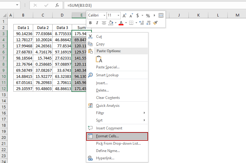
1. उन कक्षों का चयन करें जिनके लिए आप दशमलव स्थानों की संख्या सीमित करना चाहते हैं।

2. चयनित कक्षों पर राइट क्लिक करें, और चयन करें प्रारूप प्रकोष्ठों राइट-क्लिक मेनू से।

3. आने वाले फ़ॉर्मेट सेल्स डायलॉग बॉक्स में, पर जाएँ नंबर टैब पर, हाइलाइट करने के लिए क्लिक करें नंबर में वर्ग बॉक्स, और फिर उसमें एक नंबर टाइप करें दशमलव स्थान डिब्बा।
उदाहरण के लिए, यदि आप चयनित कोशिकाओं के लिए केवल 1 दशमलव स्थान सीमित करना चाहते हैं, तो बस टाइप करें 1 में दशमलव स्थान डिब्बा। नीचे स्क्रीन शॉट देखें:

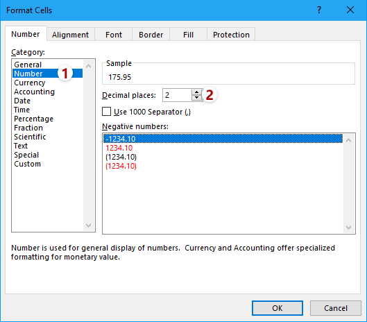
4। दबाएं OK फ़ॉर्मेट सेल संवाद बॉक्स में। फिर आप देखेंगे कि चयनित कक्षों के सभी दशमलव एक दशमलव स्थान पर बदल गए हैं।

नोट: सेलों का चयन करने के बाद, आप क्लिक कर सकते हैं दशमलव बढ़ाएँ बटन  or दशमलव घटाएं बटन  सीधे में नंबर पर समूह होम दशमलव स्थान बदलने के लिए टैब.

Excel में एकाधिक सूत्रों में दशमलव स्थानों की संख्या को आसानी से सीमित करें

सामान्य तौर पर, आप एक सूत्र में दशमलव स्थानों की संख्या को आसानी से सीमित करने के लिए =Round(original_formula, num_digits) का उपयोग कर सकते हैं। हालाँकि, कई फॉर्मूलों को एक-एक करके मैन्युअल रूप से संशोधित करना काफी कठिन और समय लेने वाला होगा। यहां, एक्सेल के लिए कुटूल की ऑपरेशन सुविधा का उपयोग करें, आप आसानी से कई सूत्रों में दशमलव स्थानों की संख्या को आसानी से सीमित कर सकते हैं!


एक्सेल के लिए कुटूल - 300 से अधिक आवश्यक उपकरणों के साथ सुपरचार्ज एक्सेल। बिना किसी क्रेडिट कार्ड की आवश्यकता के पूर्ण-विशेषताओं वाले 30-दिवसीय निःशुल्क परीक्षण का आनंद लें! अब समझे

एक्सेल में सूत्रों में दशमलव स्थानों की संख्या सीमित करें

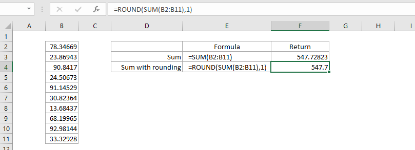
मान लीजिए कि आप संख्याओं की एक श्रृंखला के योग की गणना करते हैं, और आप सूत्र में इस योग मान के लिए दशमलव स्थानों की संख्या को सीमित करना चाहते हैं, तो आप इसे एक्सेल में कैसे कर सकते हैं? आपको राउंड फ़ंक्शन आज़माना चाहिए।

मूल गोल सूत्र सिंटैक्स है:

=गोल(संख्या, संख्या_अंक)

और यदि आप राउंड फ़ंक्शन और अन्य फ़ॉर्मूला को संयोजित करना चाहते हैं, तो फ़ॉर्मूला सिंटैक्स को बदला जाना चाहिए

=गोल(मूल_सूत्र, संख्या_अंक)

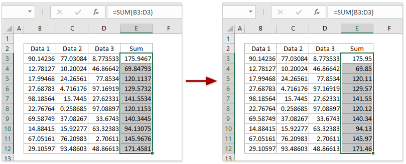
हमारे मामले में, हम योग मान के लिए एक दशमलव स्थान सीमित करना चाहते हैं, इसलिए हम नीचे दिए गए सूत्र को लागू कर सकते हैं:

=गोल(योग(बी2:बी11),1)


थोक में अनेक सूत्रों में दशमलव स्थानों की संख्या सीमित करें

यदि आपके पास एक्सेल के लिए कुटूल स्थापित, आप इसे लागू कर सकते हैं आपरेशन एकाधिक दर्ज किए गए फ़ार्मुलों को एक साथ संशोधित करने की सुविधा, जैसे एक्सेल में राउंडिंग सेट करना। कृपया इस प्रकार करें:

एक्सेल के लिए कुटूल- एक्सेल के लिए 300 से अधिक उपयोगी उपकरण शामिल हैं। पूर्ण सुविधा निःशुल्क परीक्षण 30-दिन, किसी क्रेडिट कार्ड की आवश्यकता नहीं! अब समझे

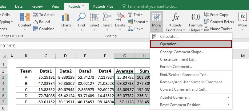
1. उन सूत्र कक्षों का चयन करें जिनके दशमलव स्थानों को आपको सीमित करना है, और क्लिक करें कुटूल > अधिक > आपरेशन.

2. ऑपरेशन टूल्स संवाद में, कृपया हाइलाइट करने के लिए क्लिक करें गोलाई में आपरेशन सूची बॉक्स में दशमलव स्थानों की संख्या टाइप करें ओपेरंड अनुभाग, और जाँच करें सूत्र बनाएँ विकल्प.
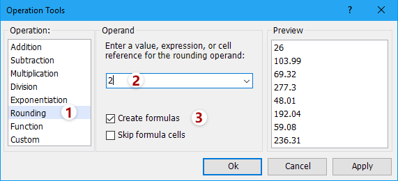
3। दबाएं Ok बटन.

अब आप देखेंगे कि सभी सूत्र कोशिकाएँ थोक में निर्दिष्ट दशमलव स्थानों पर गोल हो गई हैं। स्क्रीनशॉट देखें:

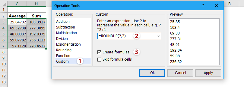
टिप: यदि आपको एक साथ कई सूत्र कक्षों को पूर्णांकित या पूर्णांकित करने की आवश्यकता है, तो आप निम्नानुसार सेट कर सकते हैं: ऑपरेशन टूल्स संवाद में, (1) चयन रिवाज ऑपरेशन सूची बॉक्स में, (2) टाइप =राउंडअप(?, 2) or =राउंडडाउन(?, 2) में रिवाज अनुभाग, और (3) चेक सूत्र बनाएँ विकल्प। स्क्रीनशॉट देखें:


Excel में एकाधिक सूत्रों में दशमलव स्थानों की संख्या को आसानी से सीमित करें

आम तौर पर दशमलव सुविधा कोशिकाओं में दशमलव स्थानों को कम कर सकती है, लेकिन फॉर्मूला बार में दिखने वाले वास्तविक मान बिल्कुल नहीं बदलते हैं। एक्सेल के लिए कुटूलहै गोल उपयोगिता आपको मानों को ऊपर/नीचे/यहां तक ​​कि निर्दिष्ट दशमलव स्थानों तक भी आसानी से गोल करने में मदद कर सकती है।

एक्सेल के लिए कुटूल- एक्सेल के लिए 300 से अधिक उपयोगी उपकरण शामिल हैं। पूर्ण सुविधा निःशुल्क परीक्षण 60-दिन, किसी क्रेडिट कार्ड की आवश्यकता नहीं! अब समझे

यह विधि सूत्र कोशिकाओं को थोक में दशमलव स्थानों की निर्दिष्ट संख्या तक गोल कर देगी। हालाँकि, यह इन सूत्र कोशिकाओं से सूत्रों को हटा देगा और केवल पूर्णांकन परिणाम ही रहेगा।


डेमो: एक्सेल में सूत्र में दशमलव स्थानों की संख्या सीमित करें

एक्सेल के लिए कुटूल: आपकी उंगलियों पर 300 से अधिक उपयोगी उपकरण! आज ही बिना किसी सुविधा सीमा के अपना 30-दिवसीय निःशुल्क परीक्षण प्रारंभ करें। अब डाउनलोड करें!

संबंधित आलेख:

सर्वोत्तम कार्यालय उत्पादकता उपकरण

🤖 कुटूल्स एआई सहयोगी: निम्न के आधार पर डेटा विश्लेषण में क्रांति लाएं: बुद्धिमान निष्पादन   |  कोड जनरेट करें  |  कस्टम फ़ॉर्मूले बनाएं  |  डेटा का विश्लेषण करें और चार्ट बनाएं  |  कुटूल फ़ंक्शंस का आह्वान करें...
लोकप्रिय सुविधाएँ: डुप्लिकेट ढूंढें, हाइलाइट करें या पहचानें   |  रिक्त पंक्तियाँ हटाएँ   |  डेटा खोए बिना कॉलम या सेल को संयोजित करें   |   फॉर्मूला के बिना गोल ...
सुपर लुकअप: एकाधिक मानदंड VLookup    मल्टीपल वैल्यू वीलुकअप  |   अनेक शीटों में VLookup   |   फजी लुकअप ....
उन्नत ड्रॉप-डाउन सूची: शीघ्रता से ड्रॉप डाउन सूची बनाएं   |  आश्रित ड्रॉप डाउन सूची   |  बहु-चयन ड्रॉप डाउन सूची ....
स्तम्भ प्रबंधक: कॉलमों की एक विशिष्ट संख्या जोड़ें  |  कॉलम ले जाएँ  |  छिपे हुए कॉलम की दृश्यता स्थिति टॉगल करें  |  रेंज और कॉलम की तुलना करें ...
फीचर्ड फीचर्स: ग्रिड फोकस   |  डिजाइन देखें   |   बड़ा फॉर्मूला बार    कार्यपुस्तिका एवं शीट प्रबंधक   |  संसाधन लाइब्रेरी (ऑटो टेक्स्ट)   |  खजूर बीनने वाला   |  कार्यपत्रकों को संयोजित करें   |  एन्क्रिप्ट/डिक्रिप्ट सेल    सूची के अनुसार ईमेल भेजें   |  सुपर फ़िल्टर   |   विशेष फ़िल्टर (फ़िल्टर बोल्ड/इटैलिक/स्ट्राइकथ्रू...) ...
शीर्ष 15 टूलसेट12 टेक्स्ट टूल्स (पाठ जोड़ें, अक्षर हटाएँ, ...)   |   50 + चार्ट प्रकार (गैन्ट चार्ट, ...)   |   40+ प्रैक्टिकल सूत्र (जन्मदिन के आधार पर आयु की गणना करें, ...)   |   19 निवेशन टूल्स (QR कोड डालें, पथ से चित्र सम्मिलित करें, ...)   |   12 रूपांतरण टूल्स (शब्दों को संख्याएँ, मुद्रा रूपांतरण, ...)   |   7 विलय और विभाजन टूल्स (उन्नत संयोजन पंक्तियाँ, विभाजन कोशिकाओं, ...)   |   ... और अधिक

एक्सेल के लिए कुटूल के साथ अपने एक्सेल कौशल को सुपरचार्ज करें, और पहले जैसी दक्षता का अनुभव करें। एक्सेल के लिए कुटूल उत्पादकता बढ़ाने और समय बचाने के लिए 300 से अधिक उन्नत सुविधाएँ प्रदान करता है।  वह सुविधा प्राप्त करने के लिए यहां क्लिक करें जिसकी आपको सबसे अधिक आवश्यकता है...

Description


ऑफिस टैब ऑफिस में टैब्ड इंटरफ़ेस लाता है, और आपके काम को बहुत आसान बनाता है

  • Word, Excel, PowerPoint में टैब्ड संपादन और रीडिंग सक्षम करें, प्रकाशक, एक्सेस, विसियो और प्रोजेक्ट।
  • नई विंडो के बजाय एक ही विंडो के नए टैब में एकाधिक दस्तावेज़ खोलें और बनाएं।
  • आपकी उत्पादकता 50% बढ़ जाती है, और आपके लिए हर दिन सैकड़ों माउस क्लिक कम हो जाते हैं!
Comments (15)
No ratings yet. Be the first to rate!
This comment was minimized by the moderator on the site
this cnu
am using excel fo milk calculations

in 1 crate having 12/lit of milk.
if customar take 12/lit in total it shows 1 using,(=number1/number2)
if customar take 24/ in total it shows 2 using,(=number1/number2)
if customar take 36/ total it shows 3using,(=number1/number2)
but some customar take 15 or 22 or 35

if customar take 15 in total it shows 1.3
if customar take 22 in total it shows 1.10
if customar take35 in total it shows 2.11

i need formula for above calculation
This comment was minimized by the moderator on the site
try this:
=roundup(number1/number2,0)
This comment was minimized by the moderator on the site
'95,954,691.3389700060
When a put this data on excel, and quit the ' to turn it a number, excel, trucante the number after 5 decimal. The new number is 95,954,691.33897, but I need 10 decimals. How to resolve this?
This comment was minimized by the moderator on the site
Try this:

=TEXT(95954691.3389100060,"00,000,000.0000000000")
This comment was minimized by the moderator on the site
Ok, here is one I really need help with since it would ease my job a lot. I have a table where i need most of my cells to have 2 decimals. One of the columns (lets say C) has to be A multiplied by B, but with a little text following the result of the multiplication, hence i gave it a:
A*B & "text" formula
My problem is that if result of A*B is 3 or 3.1 it will appear just like that: "3 text" or "3.1 text", but i really need it as "3.00 text"/ "3.10text".
Any tips?
This comment was minimized by the moderator on the site
Try this:

=TEXT(A*B,"0.00")&" text"
This comment was minimized by the moderator on the site
I want to set a limit whereas 0.60 is the threshold if the decimal reaches 0.60 it will automatically count as 1 and reset into decimal. The decimal represent the minutes and the whole number represent the hours. I'm presenting my data as numbers instead of timevalue. Hope anyone can help
This comment was minimized by the moderator on the site
Unfortunately it is not working if you concatenate:

I want to combine two cells A and B with many digits to A (B) with onlytwo digits.

I tried like that:
=CONCATENATE((ROUND(C4,1))," (",(Round(D4,1)),")")

It doesn't work and shows only the formula.
Can anyone help?
This comment was minimized by the moderator on the site
Hi yvonne Fabian,
Your formula works well in my Excel 2016.
This comment was minimized by the moderator on the site
how to deal with two decimal points e.g. 138.4622.472, 137.1416.113 etc. any way to get rid of .472 and .113 and so on
This comment was minimized by the moderator on the site
John, to round to 0 decimals, try use ROUND(CELL,0) and to round DOWN to the number, use INT (integer).
ROUND(12.5,0) = 13 ; INT(12.5) = 12
for the same but not to whole number but e.g. tenths, first multiply the baste number by 10, then ROUND/INT and then devide back by ten.
This comment was minimized by the moderator on the site
Here we are inserting the values in one cell(A1) and applying the formula in another cell(D1) (for example) and in that cell(D1) only we are getting the output , but I want to apply the formula in cell(A1) only so I can get the output in that cell (A1).
If I am doing this then I am not getting any output in the cell (A1).
Please help me to achieve this.
This comment was minimized by the moderator on the site
Hi Narsingh,
Kutools for Excel provides an Operation tools which can custom formula to selected cells. This feature may solve your problem.
This comment was minimized by the moderator on the site
Here we are inserting the values in one cell(A1) and applying the formula in another cell(D1) (for example) and in that cell(D1) only we are getting the output , but I want to apply the formula in cell(A1) only so I can get the output in that cell (A1).
If I am doing this then I am not getting any output in the cell (A1).
Please help me to achieve this.
This comment was minimized by the moderator on the site
thanks, this soo helpfull :-)
There are no comments posted here yet
Please leave your comments in English
Posting as Guest
×
Rate this post:
0   Characters
Suggested Locations