मुख्य सामग्री पर जाएं

Excel में पाठ मानदंड के आधार पर मानों का योग कैसे करें?

लेखक: ज़ियाओयांग अंतिम संशोधित: 2020-04-21

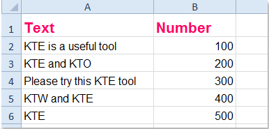
एक्सेल में, क्या आपने कभी पाठ मानदंड के किसी अन्य कॉलम के आधार पर मानों का योग करने का प्रयास किया है? उदाहरण के लिए, मेरे पास वर्कशीट में डेटा की एक श्रृंखला है जैसा कि निम्नलिखित स्क्रीनशॉट में दिखाया गया है, अब, मैं कॉलम बी में सभी संख्याओं को कॉलम ए में टेक्स्ट मानों के साथ जोड़ना चाहता हूं जो एक निश्चित मानदंड को पूरा करते हैं, जैसे संख्याओं का योग यदि कॉलम A की कोशिकाओं में KTE शामिल है।

दस्तावेज़-योग-आधारित-पर-पाठ-1

यदि कुछ पाठ शामिल है तो दूसरे कॉलम के आधार पर मानों का योग करें

यदि किसी पाठ से प्रारंभ होता है तो दूसरे कॉलम के आधार पर मानों का योग करें

यदि किसी निश्चित पाठ के साथ समाप्त होता है तो दूसरे कॉलम के आधार पर मानों का योग करें

यदि केवल निश्चित पाठ है तो दूसरे कॉलम के आधार पर मानों का योग करें


तीर नीला दायां बुलबुला यदि कुछ पाठ शामिल है तो दूसरे कॉलम के आधार पर मानों का योग करें

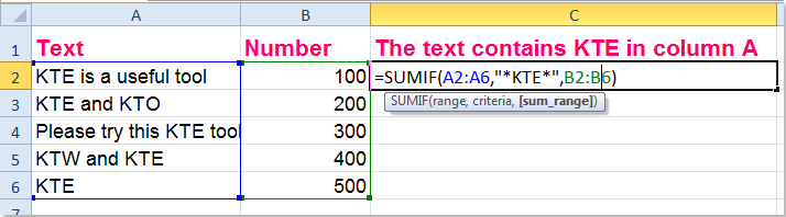
आइए उपरोक्त डेटा को उदाहरण के लिए लें, सभी मानों को एक साथ जोड़ने के लिए जिसमें कॉलम ए में "केटीई" टेक्स्ट शामिल है, निम्नलिखित सूत्र आपकी मदद कर सकता है:

कृपया यह सूत्र दर्ज करें =SUMIF(A2:A6,"*KTE*",B2:B6) एक रिक्त कक्ष में, और दबाएँ दर्ज कुंजी, फिर कॉलम बी के सभी नंबर जहां कॉलम ए में संबंधित सेल में "केटीई" टेक्स्ट है, जुड़ जाएंगे। स्क्रीनशॉट देखें:

दस्तावेज़-योग-आधारित-पर-पाठ-2
-1
दस्तावेज़-योग-आधारित-पर-पाठ-3

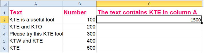
टिप: उपरोक्त सूत्र में, A2: A6 वह डेटा श्रेणी है जिसके आधार पर आप मान जोड़ते हैं, *केटीई* आपके लिए आवश्यक मानदंड को दर्शाता है, और B2:B6 वह सीमा है जिसका आप योग करना चाहते हैं।


तीर नीला दायां बुलबुला यदि किसी पाठ से प्रारंभ होता है तो दूसरे कॉलम के आधार पर मानों का योग करें

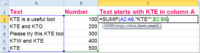
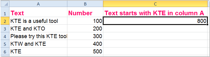
यदि आप केवल कॉलम बी में सेल मानों का योग करना चाहते हैं, जहां कॉलम ए में संबंधित सेल है, जिसका पाठ "केटीई" से शुरू होता है, तो आप इस सूत्र को लागू कर सकते हैं: =SUMIF(A2:A6,"KTE*",B2:B6), स्क्रीनशॉट देखें:

दस्तावेज़-योग-आधारित-पर-पाठ-4
-1
दस्तावेज़-योग-आधारित-पर-पाठ-5

टिप: उपरोक्त सूत्र में, A2: A6 वह डेटा श्रेणी है जिसके आधार पर आप मान जोड़ते हैं, केटीई* आपके लिए आवश्यक मानदंड को दर्शाता है, और B2:B6 वह सीमा है जिसका आप योग करना चाहते हैं।


तीर नीला दायां बुलबुला यदि किसी निश्चित पाठ के साथ समाप्त होता है तो दूसरे कॉलम के आधार पर मानों का योग करें

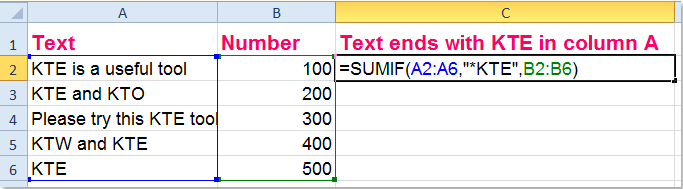
कॉलम बी में सभी मानों को जोड़ने के लिए, जहां कॉलम ए में संबंधित सेल है, जिसका पाठ "केटीई" के साथ समाप्त होता है, यह सूत्र आपकी मदद कर सकता है: =SUMIF(A2:A6,"*KTE",B2:B6)(A2: A6 वह डेटा श्रेणी है जिसके आधार पर आप मान जोड़ते हैं, केटीई* आपके लिए आवश्यक मानदंड का प्रतिनिधित्व करता है, और B2: B6 यह वह सीमा है जिसका आप योग करना चाहते हैं) स्क्रीनशॉट देखें:

दस्तावेज़-योग-आधारित-पर-पाठ-6
-1
दस्तावेज़-योग-आधारित-पर-पाठ-7

तीर नीला दायां बुलबुला यदि केवल निश्चित पाठ है तो दूसरे कॉलम के आधार पर मानों का योग करें

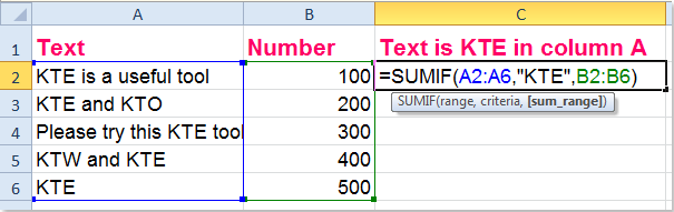
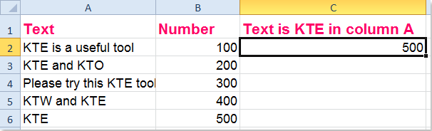
यदि आप केवल कॉलम बी में मानों का योग करना चाहते हैं, जो संबंधित सेल सामग्री केवल कॉलम ए का "केटीई" है, तो कृपया इस सूत्र का उपयोग करें: =SUMIF(A2:A6,"KTE",B2:B6)(A2: A6 वह डेटा श्रेणी है जिसके आधार पर आप मान जोड़ते हैं, केटीई आपके लिए आवश्यक मानदंड का प्रतिनिधित्व करता है, और B2: B6 वह सीमा है जिसे आप जोड़ना चाहते हैं) और उसके बाद कॉलम ए में केवल टेक्स्ट "केटीई" है, जो कॉलम बी में सापेक्ष संख्या जोड़ देगा, स्क्रीनशॉट देखें:

दस्तावेज़-योग-आधारित-पर-पाठ-8
-1
दस्तावेज़-योग-आधारित-पर-पाठ-9

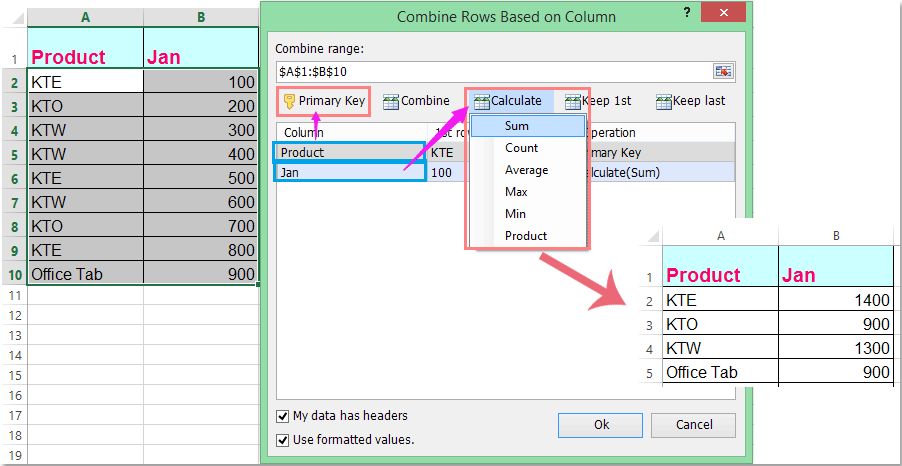
उन्नत संयोजित पंक्तियाँ: (डुप्लिकेट पंक्तियों और योग/औसत संगत मानों को संयोजित करें):
  • 1. उस कुंजी कॉलम को निर्दिष्ट करें जिसके आधार पर आप अन्य कॉलम को संयोजित करना चाहते हैं;
  • 2. अपने संयुक्त डेटा के लिए एक गणना चुनें।

दस्तावेज़-योग-कॉलम-एक-मानदंड-7

एक्सेल के लिए कुटूल: 200 से अधिक उपयोगी एक्सेल ऐड-इन्स के साथ, 60 दिनों में बिना किसी सीमा के आज़माने के लिए निःशुल्क। अभी डाउनलोड करें और निःशुल्क परीक्षण करें!


संबंधित आलेख:

Excel में प्रत्येक n पंक्तियों का योग कैसे करें?

एक्सेल में टेक्स्ट और संख्याओं के साथ सेल का योग कैसे करें?

सर्वोत्तम कार्यालय उत्पादकता उपकरण

🤖 कुटूल्स एआई सहयोगी: निम्न के आधार पर डेटा विश्लेषण में क्रांति लाएं: बुद्धिमान निष्पादन   |  कोड जनरेट करें  |  कस्टम फ़ॉर्मूले बनाएं  |  डेटा का विश्लेषण करें और चार्ट बनाएं  |  कुटूल फ़ंक्शंस का आह्वान करें...
लोकप्रिय सुविधाएँ: डुप्लिकेट ढूंढें, हाइलाइट करें या पहचानें   |  रिक्त पंक्तियाँ हटाएँ   |  डेटा खोए बिना कॉलम या सेल को संयोजित करें   |   फॉर्मूला के बिना गोल ...
सुपर लुकअप: एकाधिक मानदंड VLookup    मल्टीपल वैल्यू वीलुकअप  |   अनेक शीटों में VLookup   |   फजी लुकअप ....
उन्नत ड्रॉप-डाउन सूची: शीघ्रता से ड्रॉप डाउन सूची बनाएं   |  आश्रित ड्रॉप डाउन सूची   |  बहु-चयन ड्रॉप डाउन सूची ....
स्तम्भ प्रबंधक: कॉलमों की एक विशिष्ट संख्या जोड़ें  |  कॉलम ले जाएँ  |  छिपे हुए कॉलम की दृश्यता स्थिति टॉगल करें  |  रेंज और कॉलम की तुलना करें ...
फीचर्ड फीचर्स: ग्रिड फोकस   |  डिजाइन देखें   |   बड़ा फॉर्मूला बार    कार्यपुस्तिका एवं शीट प्रबंधक   |  संसाधन लाइब्रेरी (ऑटो टेक्स्ट)   |  खजूर बीनने वाला   |  कार्यपत्रकों को संयोजित करें   |  एन्क्रिप्ट/डिक्रिप्ट सेल    सूची के अनुसार ईमेल भेजें   |  सुपर फ़िल्टर   |   विशेष फ़िल्टर (फ़िल्टर बोल्ड/इटैलिक/स्ट्राइकथ्रू...) ...
शीर्ष 15 टूलसेट12 टेक्स्ट टूल्स (पाठ जोड़ें, अक्षर हटाएँ, ...)   |   50 + चार्ट प्रकार (गैन्ट चार्ट, ...)   |   40+ प्रैक्टिकल सूत्र (जन्मदिन के आधार पर आयु की गणना करें, ...)   |   19 निवेशन टूल्स (QR कोड डालें, पथ से चित्र सम्मिलित करें, ...)   |   12 रूपांतरण टूल्स (शब्दों को संख्याएँ, मुद्रा रूपांतरण, ...)   |   7 विलय और विभाजन टूल्स (उन्नत संयोजन पंक्तियाँ, विभाजन कोशिकाओं, ...)   |   ... और अधिक

एक्सेल के लिए कुटूल के साथ अपने एक्सेल कौशल को सुपरचार्ज करें, और पहले जैसी दक्षता का अनुभव करें। एक्सेल के लिए कुटूल उत्पादकता बढ़ाने और समय बचाने के लिए 300 से अधिक उन्नत सुविधाएँ प्रदान करता है।  वह सुविधा प्राप्त करने के लिए यहां क्लिक करें जिसकी आपको सबसे अधिक आवश्यकता है...

Description


ऑफिस टैब ऑफिस में टैब्ड इंटरफ़ेस लाता है, और आपके काम को बहुत आसान बनाता है

  • Word, Excel, PowerPoint में टैब्ड संपादन और रीडिंग सक्षम करें, प्रकाशक, एक्सेस, विसियो और प्रोजेक्ट।
  • नई विंडो के बजाय एक ही विंडो के नए टैब में एकाधिक दस्तावेज़ खोलें और बनाएं।
  • आपकी उत्पादकता 50% बढ़ जाती है, और आपके लिए हर दिन सैकड़ों माउस क्लिक कम हो जाते हैं!
Comments (22)
No ratings yet. Be the first to rate!
This comment was minimized by the moderator on the site
I try already.cause I apply the whole range it's still could not get the total sum. I am used sumif
This comment was minimized by the moderator on the site
i need to reference my sumifs criteria to a specific cell, the cell acts as a filter
EG: =SUMIFS(LV215:LV237,WC7,AB215:AB237) where WC7 is equal to a specific cell is this possible?
This comment was minimized by the moderator on the site
i cannot find this tool. "Combine Rows Based on Column" at the top of the page. i also cannot find info on what is on the free version vs. what is on the paid version. is this on the paid version? if not, where is it? thanks!
This comment was minimized by the moderator on the site
Hello, jenna,
We have moved this feature under the Merge & Split group, please see the below screenshot.
Sorry for this inconvenience.
Please try, thank you!
This comment was minimized by the moderator on the site
I create a dynamic string which contains the cells to sum and pass this string to sum function and it gives me #value error. Any solution to this.
This comment was minimized by the moderator on the site
Hi, Desu,
Could you give your problem more detailed, thank you!
This comment was minimized by the moderator on the site
By the way, I’m using the =SUMIF(A2:A6,"*KTE*",B2:B6) formula, and I want to do more than just the B column (up to column AM).
This comment was minimized by the moderator on the site
Hello, Paige,
For solving your problem, may be there is no simple formula, you should join the SUMIF function together to get the result as you need, for example, you can use the below formula: (you can add other columns data with combining the sumif function)

=SUM(SUMIF(A2:A6,"*kte*",B2:B6), SUMIF(A2:A6,"*kte*",C2:C6), SUMIF(A2:A6,"*kte*",D2:D6))

Please try it, hope it can help you!
This comment was minimized by the moderator on the site
This works but what if I want to use the last part of the formula to cover multiple columns instead of just one?
This comment was minimized by the moderator on the site
how do I use a sumif in the following. If a certain cell contains the values of an substring of data, than sum a nearby column. for example, Cell A1 has (Dan,Tom,Bill,Smith). Then a separate table has Dan - 2, Bill - 3, John - 4. Assuming that is a 2x3 table. I want to create a formula that can sum the Dan and Bill numbers (2+3) because those texts could be found in cell A1. So the total would return 5.
This comment was minimized by the moderator on the site
How do you us sumif formula to with two criteria? For instance, If Column A = X and Column C = C then Sum Column G.
This comment was minimized by the moderator on the site
Hello, Matusiak
To sumif values based on multiple criteria, please view the following screenshot:

Also, you can go to the article https://www.extendoffice.com/documents/excel/2471-excel-sumif-multiple-criteria.html to get your solution.
This comment was minimized by the moderator on the site
Hi, any one here is having an idea of how to calculate value containing in a cell (Or with text?
For Example: in Cell A= MR134 , B= MR143, C = MR187 and result will be like sum of 134+143+187 =?
This comment was minimized by the moderator on the site
I am looking for this solution too.
This comment was minimized by the moderator on the site
Hello, guys,
May be the below array formula can help you: (after typing the formula, please press Ctrl+Shift+Enter together)
=SUM(IF(ISNUMBER(SEARCH("MR",B1:B4)),SUBSTITUTE(B1:B4,"MR",""))+0)
Please change the cell references to your need.
This comment was minimized by the moderator on the site
This is super clear and understandable, thank you so much!!!
There are no comments posted here yet
Load More
Please leave your comments in English
Posting as Guest
×
Rate this post:
0   Characters
Suggested Locations