मुख्य सामग्री पर जाएं

एक्सेल में सेल वैल्यू के आधार पर बैकग्राउंड या फॉन्ट का रंग कैसे बदलें?

लेखक: केली अंतिम संशोधित: 2021-11-12

जब आप एक्सेल में विशाल डेटा के साथ काम करते हैं, तो आप कुछ मूल्य चुनना और उन्हें विशिष्ट पृष्ठभूमि या फ़ॉन्ट रंग के साथ हाइलाइट करना चाह सकते हैं। यह आलेख एक्सेल में सेल मानों के आधार पर पृष्ठभूमि या फ़ॉन्ट रंग को तुरंत बदलने के तरीके के बारे में बात कर रहा है।


विधि 1: सशर्त स्वरूपण के साथ गतिशील रूप से सेल मान के आधार पर पृष्ठभूमि या फ़ॉन्ट रंग बदलें


RSI सशर्त फॉर्मेटिंग यह सुविधा आपको x से अधिक, y से कम, या x और y के बीच के मानों को उजागर करने में मदद कर सकती है।

मान लीजिए कि आपके पास डेटा की एक श्रृंखला है, और अब आपको 80 और 100 के बीच मानों को रंगने की आवश्यकता है, तो कृपया निम्नलिखित चरणों का पालन करें:

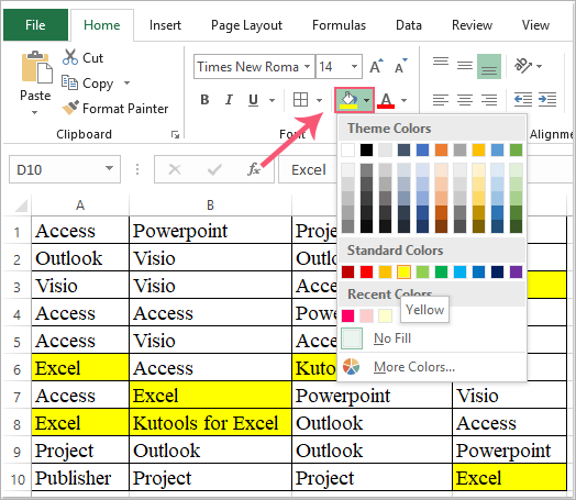
1. उन कक्षों की श्रेणी का चयन करें जिन्हें आप कुछ कक्षों को हाइलाइट करना चाहते हैं, और फिर क्लिक करें होम > सशर्त फॉर्मेटिंग > नए नियम, स्क्रीनशॉट देखें:

दस्तावेज़ मान 1 के आधार पर हाइलाइट करें

2. में नया प्रारूपण नियम संवाद बॉक्स, का चयन करें केवल उन कक्षों को प्रारूपित करें जिनमें शामिल हैं में आइटम एक नियम प्रकार चुनें बॉक्स, और में के साथ केवल सेल प्रारूपित करें अनुभाग, वे शर्तें निर्दिष्ट करें जिनकी आपको आवश्यकता है:

  • पहले ड्रॉप डाउन बॉक्स में, चुनें सेल वैल्यू;
  • दूसरे ड्रॉप डाउन बॉक्स में, मानदंड चुनें:के बीच;
  • तीसरे और चौथे बॉक्स में, फ़िल्टर स्थितियाँ दर्ज करें, जैसे 80, 100।

दस्तावेज़ मान 2 के आधार पर हाइलाइट करें

3। तब दबायें का गठन बटन, में प्रारूप प्रकोष्ठों संवाद बॉक्स में, पृष्ठभूमि या फ़ॉन्ट रंग इस प्रकार सेट करें:

सेल मान के अनुसार पृष्ठभूमि का रंग बदलें: सेल मान के अनुसार फ़ॉन्ट का रंग बदलें
क्लिक करें भरना टैब, और फिर अपनी पसंद का एक पृष्ठभूमि रंग चुनें क्लिक करें फॉन्ट टैब, और वह फ़ॉन्ट रंग चुनें जिसकी आपको आवश्यकता है।
दस्तावेज़ मान 3 के आधार पर हाइलाइट करें दस्तावेज़ मान 4 के आधार पर हाइलाइट करें

4. बैकग्राउंड या फॉन्ट कलर चुनने के बाद क्लिक करें OK > OK संवादों को बंद करने के लिए, और अब, 80 और 100 के बीच मान वाले विशिष्ट कक्षों को चयन में निश्चित पृष्ठभूमि या फ़ॉन्ट रंग में बदल दिया जाता है। स्क्रीनशॉट देखें:

पृष्ठभूमि रंग के साथ विशिष्ट कोशिकाओं को हाइलाइट करें: फ़ॉन्ट रंग के साथ विशिष्ट कक्षों को हाइलाइट करें:
दस्तावेज़ मान 5 के आधार पर हाइलाइट करें दस्तावेज़ मान 6 के आधार पर हाइलाइट करें

नोट: सशर्त फॉर्मेटिंग एक गतिशील विशेषता है, डेटा बदलते ही सेल का रंग बदल जाएगा।


विधि 2: फाइंड फ़ंक्शन के साथ सेल मान के आधार पर पृष्ठभूमि या फ़ॉन्ट रंग को स्थिर रूप से बदलें


कभी-कभी, आपको सेल मान के आधार पर एक विशिष्ट भरण या फ़ॉन्ट रंग लागू करने की आवश्यकता होती है और यह सुनिश्चित करना होता है कि सेल मान बदलने पर भरण या फ़ॉन्ट रंग न बदले। इस स्थिति में, आप इसका उपयोग कर सकते हैं खोज सभी विशिष्ट सेल मानों को खोजने के लिए फ़ंक्शन और फिर अपनी आवश्यकता के अनुसार पृष्ठभूमि या फ़ॉन्ट रंग बदलें।

उदाहरण के लिए, यदि सेल मान में "एक्सेल" टेक्स्ट है तो आप पृष्ठभूमि या फ़ॉन्ट का रंग बदलना चाहते हैं, कृपया ऐसा करें:

1. वह डेटा श्रेणी चुनें जिसका आप उपयोग करना चाहते हैं और फिर क्लिक करें होम > खोजें और चुनें > खोज, स्क्रीनशॉट देखें:

दस्तावेज़ मान 7 के आधार पर हाइलाइट करें

2. में ढूँढें और बदलें डायलॉग बॉक्स, के अंतर्गत खोज टैब में वह मान दर्ज करें जिसे आप खोजना चाहते हैं क्या पता टेक्स्ट बॉक्स, स्क्रीनशॉट देखें:

दस्तावेज़ मान 8 के आधार पर हाइलाइट करें

टिप्स: यदि आपको केस सेंसिटिव या संपूर्ण सेल सामग्री से मेल खाने वाले मान खोजने की आवश्यकता है, तो कृपया क्लिक करें ऑप्शंस उन्नत खोज विकल्प प्राप्त करने के लिए बटन, जैसे "मैच केस"और"संपूर्ण सेल सामग्री का मिलान करें" जैसी तुम्हारी ज़रूरत है।

3. और फिर, क्लिक करें सब ढूँढ़ो बटन, परिणाम खोजें बॉक्स में, किसी एक आइटम पर क्लिक करें और फिर दबाएँ Ctrl + एक सभी पाए गए आइटम का चयन करने के लिए स्क्रीनशॉट देखें:

दस्तावेज़ मान 9 के आधार पर हाइलाइट करें

4. अंत में क्लिक करें समापन इस संवाद को बंद करने के लिए बटन। अब, आप इन चयनित मानों के लिए पृष्ठभूमि या फ़ॉन्ट रंग भर सकते हैं, स्क्रीनशॉट देखें:

चयनित कक्षों के लिए पृष्ठभूमि रंग लागू करें: चयनित कक्षों के लिए फ़ॉन्ट रंग लागू करें:
दस्तावेज़ मान 10 के आधार पर हाइलाइट करें दस्तावेज़ मान 11 के आधार पर हाइलाइट करें

विधि 3: एक्सेल के लिए कुटूल के साथ सेल मान के आधार पर पृष्ठभूमि या फ़ॉन्ट रंग को स्थिर रूप से बदलें


एक्सेल के लिए कुटूलहै सुपर फाइंड यह सुविधा मानों, टेक्स्ट स्ट्रिंग्स, तिथियों, सूत्रों, स्वरूपित कोशिकाओं आदि को खोजने के लिए कई स्थितियों का समर्थन करती है। मिलान किए गए सेल ढूंढने और चुनने के बाद, आप पृष्ठभूमि या फ़ॉन्ट रंग को अपनी इच्छानुसार बदल सकते हैं।

स्थापित करने के बाद एक्सेल के लिए कुटूल, कृपया ऐसा करें:

1. वह डेटा श्रेणी चुनें जिसे आप ढूंढना चाहते हैं और फिर क्लिक करें कुटूल > सुपर फाइंड, स्क्रीनशॉट देखें:

दस्तावेज़ मान 12 के आधार पर हाइलाइट करें

2. में सुपर फाइंड फलक, कृपया निम्नलिखित कार्य करें:

  • (1.) सबसे पहले, क्लिक करें मान विकल्प चिह्न;
  • (2.) में से खोज का दायरा चुनें अंदर नीचे छोड़ें, इस मामले में, मैं चुनूंगा चयन;
  • (3.)से प्रकार ड्रॉप डाउन सूची, वह मानदंड चुनें जिसका आप उपयोग करना चाहते हैं;
  • (4.) फिर क्लिक करें खोज सभी संबंधित परिणामों को सूची बॉक्स में सूचीबद्ध करने के लिए बटन;
  • (5.) अंत में क्लिक करें चुनते हैं कक्षों का चयन करने के लिए बटन।

दस्तावेज़ मान 13 के आधार पर हाइलाइट करें

3. और फिर, मानदंड से मेल खाने वाली सभी कोशिकाओं को एक ही बार में चुना गया है, स्क्रीनशॉट देखें:

दस्तावेज़ मान 14 के आधार पर हाइलाइट करें

4. और अब, आप अपनी आवश्यकतानुसार चयनित सेल के लिए पृष्ठभूमि रंग या फ़ॉन्ट रंग बदल सकते हैं।

टिप्स: उसके साथ सुपर फाइंड फ़ंक्शन, आप निम्नलिखित परिचालनों को भी शीघ्रता और आसानी से निपटा सकते हैं:

एक्सेल में विशिष्ट मानदंड के साथ टेक्स्ट स्ट्रिंग ढूंढें और चुनें एक्सेल में विशिष्ट मानदंडों के आधार पर दिनांक सेल ढूंढें और चुनें
एक्सेल में टिप्पणियों के भीतर विशिष्ट टेक्स्ट स्ट्रिंग ढूंढें और चुनें एक्सेल में सूत्रों के भीतर विशिष्ट टेक्स्ट स्ट्रिंग ढूंढें और चुनें
एक्सेल में हाइपरलिंक के भीतर विशिष्ट टेक्स्ट स्ट्रिंग ढूंढें और चुनें एक्सेल में विशिष्ट सेल फ़ॉर्मेटिंग वाले सभी सेल ढूंढें और चुनें

अधिक पढ़ें...             डाउनलोड करें और 60 दिन का निःशुल्क परीक्षण करें


सप्ताहांत पर व्यस्त कार्य, उपयोग एक्सेल के लिए कुटूल,
आपको एक आरामदायक और आनंदमय सप्ताहांत देता है!

सप्ताहांत में, बच्चे खेलने के लिए बाहर जाने के लिए उत्सुक रहते हैं, लेकिन आपके चारों ओर इतना काम होता है कि परिवार के साथ समय बिताने के लिए समय नहीं मिल पाता। सूरज, समुद्र तट और समुद्र इतनी दूर? एक्सेल के लिए कुटूल तुम में मदद करता है एक्सेल पहेलियाँ हल करें, काम का समय बचाएं।

तस्वीर समुद्रतट
  •  प्रमोशन मिलना और सैलरी बढ़ना तो दूर की बात नहीं;
  •  इसमें उन्नत सुविधाएँ शामिल हैं, एप्लिकेशन परिदृश्यों को हल करें, कुछ सुविधाएँ 99% कार्य समय भी बचाती हैं;
  •  3 मिनट में एक्सेल विशेषज्ञ बनें, और अपने सहकर्मियों या दोस्तों से पहचान प्राप्त करें;
  •  अब Google से समाधान खोजने की ज़रूरत नहीं है, दर्दनाक फ़ार्मुलों और VBA कोड को अलविदा कहें;
  •  दोहराए गए सभी ऑपरेशन केवल कुछ क्लिक के साथ पूरे किए जा सकते हैं, अपने थके हुए हाथों को मुक्त करें;
  •  केवल $39 लेकिन अन्य लोगों के $4000 एक्सेल ट्यूटोरियल से अधिक मूल्यवान;
  •  110,000 अभिजात वर्ग और 300 से अधिक प्रसिद्ध कंपनियों द्वारा चुना जाए;
  •  30-दिन का निःशुल्क परीक्षण, और बिना किसी कारण के 60-दिन के भीतर पूरा पैसा वापस;
  •  अपने काम करने का तरीका बदलें और फिर अपनी जीवन शैली बदलें!
 

Comments (79)
No ratings yet. Be the first to rate!
This comment was minimized by the moderator on the site
Good Day,

I have a schedule with different course modules that can be placed in different order ( 1 is metal, 2 is machining, 3 is refinishing, etc.) depending on course director preferences and staff availability.

What I am trying to do to wrap up the spreadsheet is color code the modules across the months based on their order in the overall course. So if Metal is first and is 35 days long, the first 35 days are background colored blue, but if machining is first and is 20 days long, then the first 20 days are purple.

How can you do and if statement that refers to a separate cell for the initial number of days, AND color the cells based on the range between 1 and 20 or 35 or whatever?

Can I do a conditional formatting If statement with a range between numbers?

This would have to be applied to all the modules (therefor multiple conditional formatting formulas) to account for any module being in any place in the order.
That is the issue I have. Please offer any suggestions. Note that I have built the spreadsheet without VBA. (I've never had the opportunity to learn it)
This comment was minimized by the moderator on the site
Can I give colour for a row of values with respect to previous value for a whole row.
Eg

23

45

32

56

can I give red for 23 and green for 45 and again red for 32 as it is less than the previous value and green for 56 as it is more than 32.
This comment was minimized by the moderator on the site
I do get to change a cell colour according to the text or letter in fill in the cell e.g.-H=YELLOW,E=GREEN
This comment was minimized by the moderator on the site
Hello, VANESSA,
For solving your problem, please apply the Conditional Formatting feature, in the New Formatting Rule dialog box, choose the conditions as following screenshot shown:
This comment was minimized by the moderator on the site
how do i change the colour of cell depending on what is in that cell IE. Y=green N=red.

thats how i need it if it has Y riten in the cell it turns green?
This comment was minimized by the moderator on the site
Hello, Leon,
To highlight the cells based on the cell value, you should apply the Conditional Formatting feature, go to the New Formatting Rule dialog box, and then do as the following screenshot shown to highlight the cells which are Y located as green:

Do with the same way to format the cells N as red color.

Please try it, hope it can help you!
This comment was minimized by the moderator on the site
Trying to get a cell to highlight if its above a certain number, the problem is that the cell includes the number and a date. Is there a way i can get it to just look at the number? The cell will include a number+date.....1400(7/2/2018). I need the formulate just to look at the 1400 and not the date.
any ideas?
thanks
Z
This comment was minimized by the moderator on the site
Sir, I have value in cell A10, in A12. Now I entered a simple formula in A15 subtracting these (A10-A12). I want background color of result cell (A15) in green if A10 is large (means result in positive number) and background color in red if A12 is large ( result in negative number). Please provide solution
This comment was minimized by the moderator on the site
Hello,
You can select the formula cells, and then apply the Conditional Formatting > Greater than (0)-format it green, and then Less Than (0)-format it red, see screenshot:

Please try it, hope it can help you, thank you!
This comment was minimized by the moderator on the site
If I have a date in a cell, how do I make it change to orange when it is within 30 days of coming due, yellow when it is within 15 days of coming due and red when it exceeds the date (past due)
This comment was minimized by the moderator on the site
I thought this color of cells by value was going to be a real pain. It could not have been explained more easily and clearly. Thanks. It took no less than 1-2 minutes to understand what to do.
This comment was minimized by the moderator on the site
HI, I want if i change any value or number in any cell then that cell text color should get change for e.g. if number in any cell is 100 and I have to change it as 98 then that cell text 98 should change into red color. Is it possible in Excel?? Do clarify please
This comment was minimized by the moderator on the site
So I am creating a excel spreadsheet for fire department reports. What I am looking for is it to calculate the days a report is overdue, unless it has been completed: Column A Column B Column C Column D Column E Column F Incident # Incident Date Todays Date Completed Date Days Overdue Todays Date I want column B subtracting Column C to calculate in column E unless Column D is complete. I hope this makes sense. I want to use the conditional formatting to show me in colors how long a report is overdue (with the 3 color scale). I have the formula for the number of days it is overdue to have a correct value and color scale, but I want it to remain green when the report has been completed.
There are no comments posted here yet
Load More
Please leave your comments in English
Posting as Guest
×
Rate this post:
0   Characters
Suggested Locations